8 Introduction to randomization, Part 1
2.0
8.1 Introduction
In this module, we’ll learn about randomization and simulation. When we want to understand how sampling works, it’s helpful to simulate the process of drawing samples repeatedly from a population. In the days before computing, this was very difficult to do. Now, a few simple lines of computer code can generate thousands (even millions) of random samples, often in a matter of seconds or less.
8.1.1 Install new packages
If you are using RStudio Workbench, you do not need to install any packages. (Any packages you need should already be installed by the server administrators.)
If you are using R and RStudio on your own machine instead of accessing RStudio Workbench through a browser, you’ll need to type the following command at the Console:
install.packages("mosaic")8.1.2 Download the R notebook file
Check the upper-right corner in RStudio to make sure you’re in your intro_stats project. Then click on the following link to download this chapter as an R notebook file (.Rmd).
https://vectorposse.github.io/intro_stats/chapter_downloads/08-intro_to_randomization_1.Rmd
Once the file is downloaded, move it to your project folder in RStudio and open it there.
8.1.3 Restart R and run all chunks
In RStudio, select “Restart R and Run All Chunks” from the “Run” menu.
8.1.4 Load packages
We load the tidyverse package. The mosaic package contains some tools for making it easier to learn about randomization and simulation.
## ── Attaching core tidyverse packages ──────────────────────── tidyverse 2.0.0 ──
## ✔ dplyr     1.1.2     ✔ readr     2.1.4
## ✔ forcats   1.0.0     ✔ stringr   1.5.0
## ✔ ggplot2   3.4.2     ✔ tibble    3.2.1
## ✔ lubridate 1.9.2     ✔ tidyr     1.3.0
## ✔ purrr     1.0.2
## ── Conflicts ────────────────────────────────────────── tidyverse_conflicts() ──
## ✖ dplyr::filter() masks stats::filter()
## ✖ dplyr::lag()    masks stats::lag()
## ℹ Use the conflicted package (<http://conflicted.r-lib.org/>) to force all conflicts to become errors## Warning: package 'mosaic' was built under R version 4.3.1## Registered S3 method overwritten by 'mosaic':
## method from
## fortify.SpatialPolygonsDataFrame ggplot2
##
## The 'mosaic' package masks several functions from core packages in order to add
## additional features. The original behavior of these functions should not be affected by this.
##
## Attaching package: 'mosaic'
##
## The following object is masked from 'package:Matrix':
##
## mean
##
## The following objects are masked from 'package:dplyr':
##
## count, do, tally
##
## The following object is masked from 'package:purrr':
##
## cross
##
## The following object is masked from 'package:ggplot2':
##
## stat
##
## The following objects are masked from 'package:stats':
##
## binom.test, cor, cor.test, cov, fivenum, IQR, median, prop.test,
## quantile, sd, t.test, var
##
## The following objects are masked from 'package:base':
##
## max, mean, min, prod, range, sample, sum8.2 Sample and population
The goal of the next few chapters is to help you think about the process of sampling from a population. What do these terms mean?
A population is a group of objects we would like to study. If that sounds vague, that’s because it is. A population can be a group of any size and of any type of thing in which we’re interested. Often, populations refer to groups of people. For example, in an election, the population of interest is all voters. But if you’re a biologist, you might study populations of other kinds of organisms. If you’re an engineer, you might study populations of bolts on bridges. If you’re in finance, you might study populations of loans.
Populations are usually inaccessible in their entirety. It is impossible to survey every voter in any reasonably sized election, for example. Therefore, to study them, we have to collect a sample. A sample is a subset of the population. We might conduct a poll of 2000 voters to try to learn about voting intentions for the entire population. Of course, for that to work, the sample has to be representative of its population. We’ll have more to say about that in the future.
8.3 Flipping a coin
Before we talk about how samples are obtained from populations in the real world, we’re going to perform some simulations.
One of the simplest acts to simulate is flipping a coin. We could get an actual coin and physically flip it over and over again, but that is time-consuming and annoying. It is much easier to flip a “virtual” coin inside the computer. One way to accomplish this in R is to use the rflip command from the mosaic package. To make sure we’re flipping a fair coin, we’ll say that we want a 50% chance of heads by including the parameter prob = 0.5.
One more bit of technical detail. Since there will be some randomness involved here, we will need to include an R command to ensure that we all get the same results every time this code runs. This is called “setting the seed”. Don’t worry too much about what this is doing under the hood. The basic idea is that two people who start with the same seed will generate the same sequence of “random” numbers.
The seed 1234 in the chunk below is totally arbitrary. It could have been any number at all. (And, in fact, we’ll use different numbers just for fun.) If you change the seed, you will get different output, so we all need to use the same seed. But the actual common value we all use for the seed is irrelevant.
Here is one coin flip with a 50% chance of coming up heads:
##
## Flipping 1 coin [ Prob(Heads) = 0.5 ] ...
##
## T
##
## Number of Heads: 0 [Proportion Heads: 0]
Here are ten coin flips, each with a 50% chance of coming up heads:
##
## Flipping 10 coins [ Prob(Heads) = 0.5 ] ...
##
## T H H H H H T T H H
##
## Number of Heads: 7 [Proportion Heads: 0.7]
Just to confirm that this is a random process, let’s flip ten coins again (but without setting the seed again):
rflip(10, prob = 0.5)##
## Flipping 10 coins [ Prob(Heads) = 0.5 ] ...
##
## H H T H T H T T T T
##
## Number of Heads: 4 [Proportion Heads: 0.4]If we return to the previous seed of 1234, we should obtain the same ten coin flips we did at first:
##
## Flipping 10 coins [ Prob(Heads) = 0.5 ] ...
##
## T H H H H H T T H H
##
## Number of Heads: 7 [Proportion Heads: 0.7]
And just to see the effect of setting a different seed:
##
## Flipping 10 coins [ Prob(Heads) = 0.5 ] ...
##
## H H H T H H T H H H
##
## Number of Heads: 8 [Proportion Heads: 0.8]8.4 Multiple simulations
Suppose now that you are not the only person flipping coins. Suppose a bunch of people in a room are all flipping coins. We’ll start with ten coin flips per person, a task that could be reasonably done even without a computer.
You might observe three heads in ten flips. Fine, but what about everyone else in the room? What numbers of heads will they see?
The do command from mosaic is a way of doing something multiple times. Imagine there are twenty people in the room, each flipping a coin ten times, each time with a 50% probability of coming up heads. Observe:
The syntax could not be any simpler: do(20) * means, literally, “do twenty times.” In other words, this command is telling R to repeat an action twenty times, where the action is flipping a single coin ten times.
You’ll notice that in place of a list of outcomes (H or T) of all the individual flips, we have instead a summary of the number of heads and tails each person sees. Each row represents a person, and the columns give information about each person’s flips. (There are n = 10 flips for each person, but then the number of heads/tails—and the corresponding “proportion” of heads—changes from person to person.)
Looking at the above rows and columns, we see that the output of our little coin-flipping experiment is actually stored in a data frame! Let’s give it a name and work with it.
It is significant that we can store our outcomes this way. Because we have a data frame, we can apply all our data analysis tools (graphs, charts, tables, summary statistics, etc.) to the “data” generated from our set of simulations.
For example, what is the mean number of heads these twenty people observed?
mean(coin_flips_20_10$heads)## [1] 5.6Exercise 2
The data frame coin_flips_20_10 contains four variables: n, heads, tails, and prop. In the code chunk above, we calculated mean(coin_flips_20_10$heads) which gave us the mean count of heads for all people flipping coins. Instead of calculating the mean count of heads, change the variable from heads to prop to calculate the mean proportion of heads. Then explain why your answer makes sense in light of the mean count of heads calculated above.
# Add code here to calculate the mean proportion of heads.Please write up your answer here.
Let’s look at a histogram of the number of heads we see in the simulated flips. (The fancy stuff in scale_x_continuous is just making sure that the x-axis goes from 0 to 10 and that the tick marks appear on each whole number.)
ggplot(coin_flips_20_10, aes(x = heads)) +
    geom_histogram(binwidth = 0.5) +
    scale_x_continuous(limits = c(-1, 11), breaks = seq(0, 10, 1))
## Warning: Removed 2 rows containing missing values (`geom_bar()`).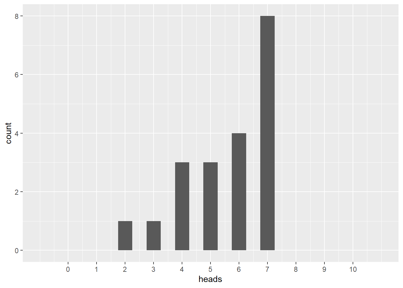
Let’s do the same thing, but now let’s consider the proportion of heads.
ggplot(coin_flips_20_10, aes(x = prop)) +
    geom_histogram(binwidth = 0.05) +
    scale_x_continuous(limits = c(-0.1, 1.1), breaks = seq(0, 1, 0.1))
## Warning: Removed 2 rows containing missing values (`geom_bar()`).
8.5 Bigger and better!
With only twenty people, it was possible that, for example, nobody would get all heads or all tails. Indeed, in coin_flips_20_10 there were no people who got all heads or all tails. Also, there were more people with six and seven heads than with five heads, even though we “expected” the average to be five heads. There is nothing particularly significant about that; it happened by pure chance alone. Another run through the above commands would generate a somewhat different outcome. That’s what happens when things are random.
Instead, let’s imagine that we recruited way more people to flip coins with us. Let’s try it again with 2000 people:
This is the same idea as before, but now there are 2000 rows in the data frame instead of 20.
mean(coin_flips_2000_10$heads)## [1] 5.0245
ggplot(coin_flips_2000_10, aes(x = heads)) +
    geom_histogram(binwidth = 0.5) +
    scale_x_continuous(limits = c(-1, 11), breaks = seq(0, 10, 1))
## Warning: Removed 2 rows containing missing values (`geom_bar()`).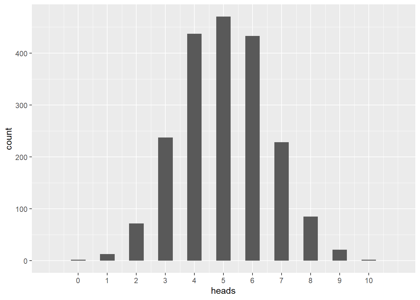
This is helpful. In contrast with the set of simulations with twenty people, the last histogram gives us something closer to what we expect. The mode is at five heads, and every possible number of heads is represented, with decreasing counts as one moves away from five. With 2000 people flipping coins, all possible outcomes—including rare ones—are better represented.
Here is the the same histogram, but this time with the proportion of heads instead of the count of heads:
ggplot(coin_flips_2000_10, aes(x = prop)) +
    geom_histogram(binwidth = 0.05) +
    scale_x_continuous(limits = c(-0.1, 1.1), breaks = seq(0, 1, 0.1))
## Warning: Removed 2 rows containing missing values (`geom_bar()`).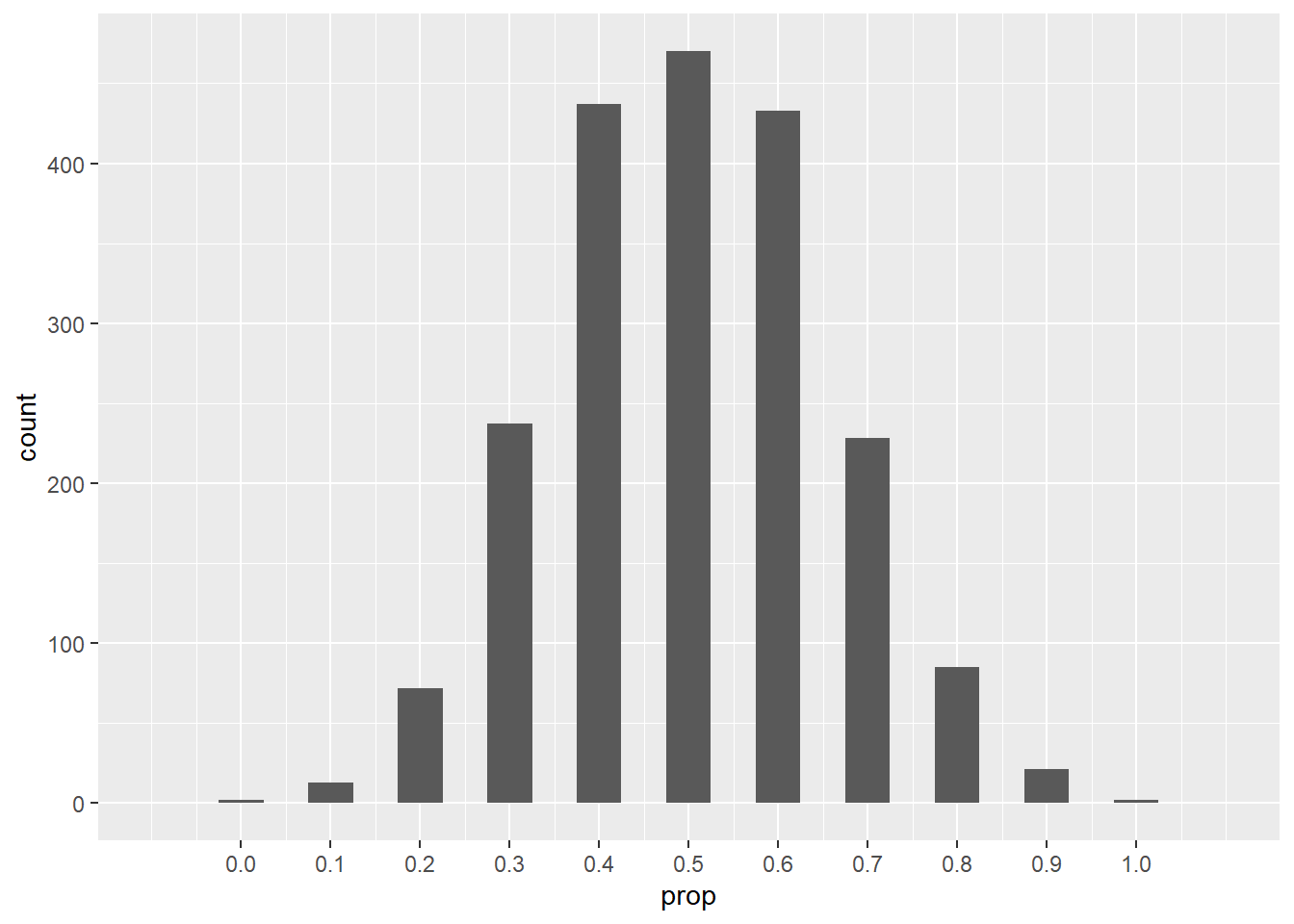
Exercise 3
Do you think the shape of the distribution would be appreciably different if we used 20,000 or even 200,000 people? Why or why not? (Normally, I would encourage you to test your theory by trying it in R. However, it takes a long time to simulate that many flips and I don’t want you to tie up resources and memory. Think through this in your head.)
Please write up your answer here.
From now on, we will insist on using at least a thousand simulations—if not more—to make sure that we represent the full range of possible outcomes.10
8.6 More flips
Now let’s increase the number of coin flips each person performs. We’ll still use 2000 simulations (imagine 2000 people all flipping coins), but this time, each person will flip the coin 1000 times instead of only 10 times. The first code chunk below accounts for a substantial amount of the time it takes to run the code in this document.
mean(coin_flips_2000_1000$heads)## [1] 499.9055
ggplot(coin_flips_2000_1000, aes(x = heads)) +
    geom_histogram(binwidth = 10, boundary = 500)
And now the same histogram, but with proportions:
ggplot(coin_flips_2000_1000, aes(x = prop)) +
    geom_histogram(binwidth = 0.01, boundary = 0.5)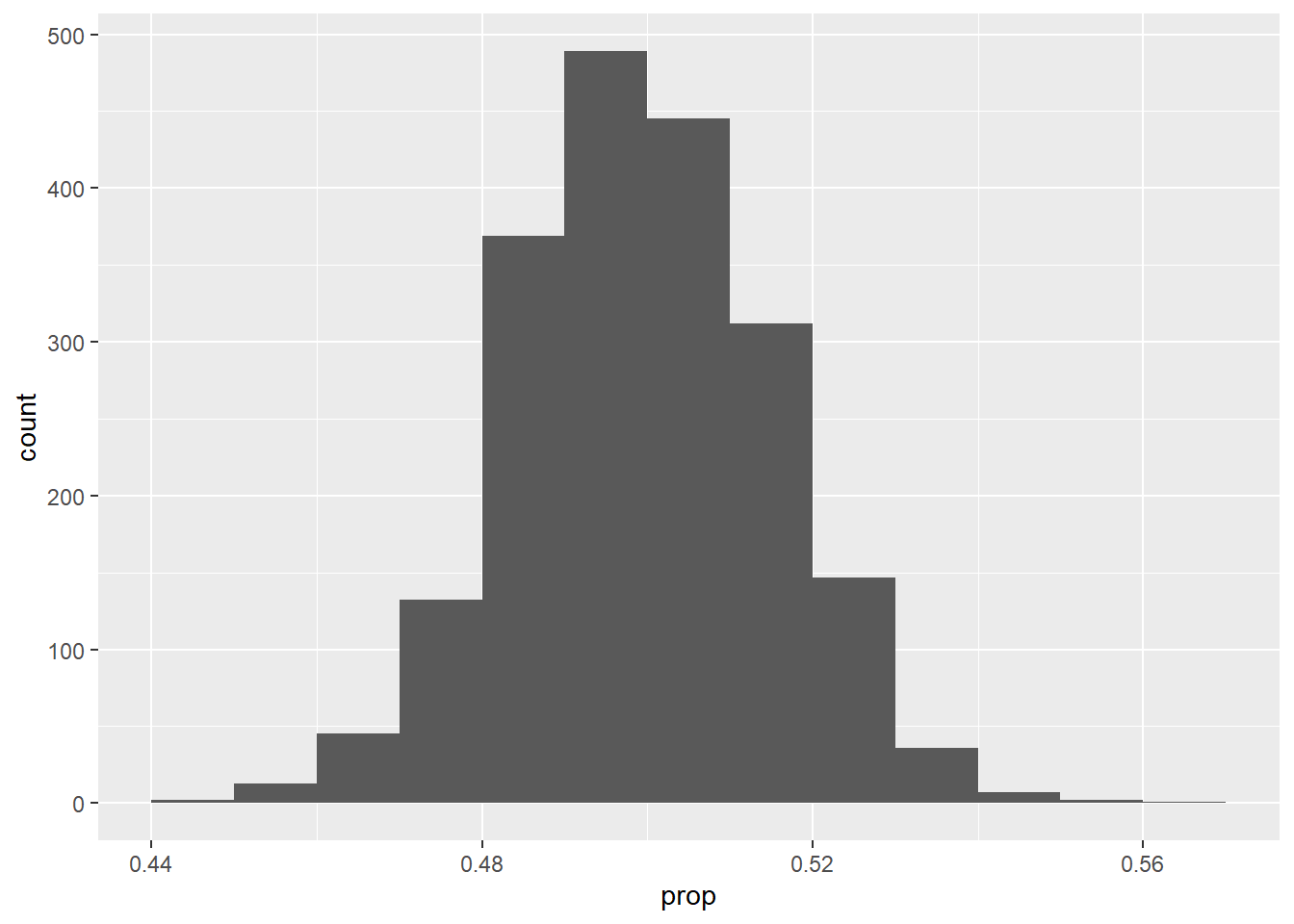
8.7 But who cares about coin flips?
It’s fair to ask why we go to all this trouble to talk about coin flips. The most pressing research questions of our day do not involve people sitting around and flipping coins, either physically or virtually.
But now substitute “heads” and “tails” with “cancer” and “no cancer”. Or “guilty” and “not guilty”. Or “shot” and “not shot”. The fact is that many important issues are measured as variables with two possible outcomes. There is some underlying “probability” of seeing one outcome over the other. (It doesn’t have to be 50% like the coin.) Statistical methods—including simulation—can say a lot about what we “expect” to see if these outcomes are truly random. More importantly, when we see outcomes that aren’t consistent with our simulations, we may wonder if there is some underlying mechanism that may be not so random after all. It may not look like it on first blush, but this idea is at the core of the scientific method.
For example, let’s suppose that 85% of U.S. adults support some form of background checks for gun buyers.11 Now, imagine we went out and surveyed a random group of people and asked them a simple yes/no question about their support for background checks. What might we see?
Let’s simulate. Imagine flipping a coin, but instead of coming up heads 50% of the time, suppose it were possible for the coin to come up heads 85% of the time.12 A sequence of heads and tails with this weird coin would be much like randomly surveying people and asking them about background checks.
We can make a “virtual” weird coin with the rflip command by specifying how often we want heads to come up.
##
## Flipping 1 coin [ Prob(Heads) = 0.85 ] ...
##
## H
##
## Number of Heads: 1 [Proportion Heads: 1]
If we flip our weird coin a bunch of times, we can see that our coin is not fair. Indeed, it appears to come up heads way more often than not:
##
## Flipping 100 coins [ Prob(Heads) = 0.85 ] ...
##
## H H H H T H H H H H H H H T H H H H H H H H H H H H H T H H H H H H H H
## H H T H H H H H H H H H H H H H H H H H H H H H T H H H H H H H H H H T
## H H H H H H H H T H H H H T H H H T H T H H H H H H H H
##
## Number of Heads: 90 [Proportion Heads: 0.9]
The results from the above code can be thought of as a survey of 100 random U.S. adults about their support for background checks for purchasing guns. “Heads” means “supports” and “tails” means “opposes.” If the majority of Americans support background checks, then we will come across more people in our survey who tell us they support background checks. This shows up in our simulation as the appearance of more heads than tails.
Note that there is no guarantee that our sample will have exactly 85% heads. In fact, it doesn’t; it has 90% heads.
Again, keep in mind that we’re simulating the act of obtaining a random sample of 100 U.S. adults. If we get a different sample, we’ll get different results. (We set a different seed here. That ensures that this code chunk is randomly different from the one above.)
##
## Flipping 100 coins [ Prob(Heads) = 0.85 ] ...
##
## H H H H H H H H T H H H T T T T T H H H H H H H H H T T T H H T H H H H
## T T H H H H T H H H H H H H H H H T H T H H H H H H H H H H H H H H H H
## T H H H T H H H H H H T H H H H H H H H H H H H T H H H
##
## Number of Heads: 81 [Proportion Heads: 0.81]
See, this time, only 81% came up heads, even though we expected 85%. That’s how randomness works.
Exercise 6(a)
Now imagine that 2000 people all go out and conduct surveys of 100 random U.S. adults, asking them about their support for background checks. Write some R code that simulates this. Plot a histogram of the results. (Hint: you’ll need do(2000) * in there.) Use the proportion of supporters (prop), not the raw count of supporters (heads).
set.seed(1234)
# Add code here to simulate 2000 surveys of 100 U.S. adults.
# Plot the results in a histogram using proportions.Exercise 6(b)
Run another simulation, but this time, have each person survey 1000 adults and not just 100.
set.seed(1234)
# Add code here to simulate 2000 surveys of 1000 U.S. adults.
# Plot the results in a histogram using proportions.8.8 Sampling variability
We’ve seen that taking repeated samples (using the do command) leads to lots of different outcomes. That is randomness in action. We don’t expect the results of each survey to be exactly the same every time the survey is administered.
But despite this randomness, there is an interesting pattern that we can observe. It has to do with the number of times we flip the coin. Since we’re using coin flips to simulate the act of conducting a survey, the number of coin flips is playing the role of the sample size. In other words, if we want to simulate a survey of U.S. adults with a sample size of 100, we simulate that by flipping 100 coins.
Exercise 7
Go back and look at all the examples above. What do you notice about the range of values on the x-axis when the sample size is small versus large? (In other words, in what way are the histograms different when using rflip(10, prob = ...) or rflip(100, prob = ...) versus rflip(1000, prob = ...)? It’s easier to compare histograms one to another when looking at the proportions instead of the raw head counts because proportions are always on the same scale from 0 to 1.)
Please write up your answer here.
8.9 Conclusion
Simulation is a tool for understanding what happens when a statistical process is repeated many times in a randomized way. The availability of fast computer processing makes simulation easy and accessible. Eventually, the goal will be to use simulation to answer important questions about data and the processes in the world that generate data. This is possible because, despite the ubiquitous presence of randomness, a certain order emerges when the number of samples is large enough. Even though there is sampling variability (different random outcomes each time we sample), there are patterns in that variability that can be exploited to make predictions.