22 ANOVA
2.0
22.1 Introduction
ANOVA stands for “Analysis of Variance”. In this chapter, we will study the most basic form of ANOVA, called “one-way ANOVA”. We’ve already considered the one-sample and two-sample t tests for means. ANOVA is what you do when you want to compare means for three or more groups.
22.1.1 Install new packages
If you are using R and RStudio on your own machine instead of accessing RStudio Workbench through a browser, you’ll need to type the following command at the Console:
install.packages("quantreg")22.1.2 Download the R notebook file
Check the upper-right corner in RStudio to make sure you’re in your intro_stats project. Then click on the following link to download this chapter as an R notebook file (.Rmd).
https://vectorposse.github.io/intro_stats/chapter_downloads/22-anova.Rmd
Once the file is downloaded, move it to your project folder in RStudio and open it there.
22.2 Load packages
We load the standard tidyverse, janitor, and infer packages. The quantreg package contains the uis data (which must be explicitly loaded using the data command) and the palmerpenguins package for the penguins data.
## ── Attaching core tidyverse packages ──────────────────────── tidyverse 2.0.0 ──
## ✔ dplyr     1.1.2     ✔ readr     2.1.4
## ✔ forcats   1.0.0     ✔ stringr   1.5.0
## ✔ ggplot2   3.4.2     ✔ tibble    3.2.1
## ✔ lubridate 1.9.2     ✔ tidyr     1.3.0
## ✔ purrr     1.0.2
## ── Conflicts ────────────────────────────────────────── tidyverse_conflicts() ──
## ✖ dplyr::filter() masks stats::filter()
## ✖ dplyr::lag()    masks stats::lag()
## ℹ Use the conflicted package (<http://conflicted.r-lib.org/>) to force all conflicts to become errors##
## Attaching package: 'janitor'
##
## The following objects are masked from 'package:stats':
##
## chisq.test, fisher.test## Warning: package 'quantreg' was built under R version 4.3.1## Loading required package: SparseM
##
## Attaching package: 'SparseM'
##
## The following object is masked from 'package:base':
##
## backsolve
data(uis)
library(palmerpenguins)
## Warning: package 'palmerpenguins' was built under R version 4.3.122.3 Research question
The uis data set from the quantreg package contains data from the UIS Drug Treatment Study. Is a history of IV drug use associated with depression?
Exercise 1
The help file for the uis data is particularly uninformative. The source, like so many we see in R packages, is a statistics textbook. If you happen to have access to a copy of the textbook, it’s pretty easy to look it up and see what the authors say about it. But it’s not likely you have such access.
See if you can find out more about where the data came from. This is tricky and you’re going have to dig deep.
Hint #1: Your first hits will be from the University of Illinois-Springfield. That is not the correct source.
Hint #2: You may have more success finding sources that quote from the textbook and mention more detail about the data as it’s explained in the textbook. In fact, you might even stumble across actual pages from the textbook with the direct explanation, but that is much harder. You should not try to find and download PDF files of the book itself. Not only is that illegal, but it might also come along with nasty computer viruses.
Please write up your answer here.
22.4 Data preparation and exploration
Let’s look at the UIS data:
uis
glimpse(uis)## Rows: 575
## Columns: 18
## $ ID <dbl> 1, 2, 3, 4, 5, 6, 7, 8, 9, 10, 12, 13, 14, 15, 16, 17, 18, 19, …
## $ AGE <dbl> 39, 33, 33, 32, 24, 30, 39, 27, 40, 36, 38, 29, 32, 41, 31, 27,…
## $ BECK <dbl> 9.000, 34.000, 10.000, 20.000, 5.000, 32.550, 19.000, 10.000, 2…
## $ HC <dbl> 4, 4, 2, 4, 2, 3, 4, 4, 2, 2, 2, 3, 3, 1, 1, 2, 1, 4, 3, 2, 3, …
## $ IV <dbl> 3, 2, 3, 3, 1, 3, 3, 3, 3, 3, 3, 1, 3, 3, 3, 3, 3, 2, 1, 3, 1, …
## $ NDT <dbl> 1, 8, 3, 1, 5, 1, 34, 2, 3, 7, 8, 1, 2, 8, 1, 3, 6, 1, 15, 5, 1…
## $ RACE <dbl> 0, 0, 0, 0, 1, 0, 0, 0, 0, 0, 0, 0, 1, 0, 0, 0, 0, 0, 1, 0, 0, …
## $ TREAT <dbl> 1, 1, 1, 0, 1, 1, 1, 1, 1, 1, 1, 1, 1, 1, 1, 1, 1, 1, 1, 1, 0, …
## $ SITE <dbl> 0, 0, 0, 0, 0, 0, 0, 0, 0, 0, 0, 0, 0, 0, 0, 0, 0, 0, 0, 0, 0, …
## $ LEN.T <dbl> 123, 25, 7, 66, 173, 16, 179, 21, 176, 124, 176, 79, 182, 174, …
## $ TIME <dbl> 188, 26, 207, 144, 551, 32, 459, 22, 210, 184, 212, 87, 598, 26…
## $ CENSOR <dbl> 1, 1, 1, 1, 0, 1, 1, 1, 1, 1, 1, 1, 0, 1, 1, 1, 1, 1, 1, 1, 0, …
## $ Y <dbl> 5.236442, 3.258097, 5.332719, 4.969813, 6.311735, 3.465736, 6.1…
## $ ND1 <dbl> 5.0000000, 1.1111111, 2.5000000, 5.0000000, 1.6666667, 5.000000…
## $ ND2 <dbl> -8.0471896, -0.1170672, -2.2907268, -8.0471896, -0.8513760, -8.…
## $ LNDT <dbl> 0.6931472, 2.1972246, 1.3862944, 0.6931472, 1.7917595, 0.693147…
## $ FRAC <dbl> 0.68333333, 0.13888889, 0.03888889, 0.73333333, 0.96111111, 0.0…
## $ IV3 <dbl> 1, 0, 1, 1, 0, 1, 1, 1, 1, 1, 1, 0, 1, 1, 1, 1, 1, 0, 0, 1, 0, …To talk about the ANOVA procedure, we’ll use the BECK and IV variables. We need to convert IV to a factor variable first (using the help file for guidance). We’ll add it to a new tibble called uis2.
uis2 <- uis %>%
  mutate(IV_fct = factor(IV, levels = c(1, 2, 3),
                         labels = c("Never", "Previous", "Recent")))
uis2
glimpse(uis2)## Rows: 575
## Columns: 19
## $ ID <dbl> 1, 2, 3, 4, 5, 6, 7, 8, 9, 10, 12, 13, 14, 15, 16, 17, 18, 19, …
## $ AGE <dbl> 39, 33, 33, 32, 24, 30, 39, 27, 40, 36, 38, 29, 32, 41, 31, 27,…
## $ BECK <dbl> 9.000, 34.000, 10.000, 20.000, 5.000, 32.550, 19.000, 10.000, 2…
## $ HC <dbl> 4, 4, 2, 4, 2, 3, 4, 4, 2, 2, 2, 3, 3, 1, 1, 2, 1, 4, 3, 2, 3, …
## $ IV <dbl> 3, 2, 3, 3, 1, 3, 3, 3, 3, 3, 3, 1, 3, 3, 3, 3, 3, 2, 1, 3, 1, …
## $ NDT <dbl> 1, 8, 3, 1, 5, 1, 34, 2, 3, 7, 8, 1, 2, 8, 1, 3, 6, 1, 15, 5, 1…
## $ RACE <dbl> 0, 0, 0, 0, 1, 0, 0, 0, 0, 0, 0, 0, 1, 0, 0, 0, 0, 0, 1, 0, 0, …
## $ TREAT <dbl> 1, 1, 1, 0, 1, 1, 1, 1, 1, 1, 1, 1, 1, 1, 1, 1, 1, 1, 1, 1, 0, …
## $ SITE <dbl> 0, 0, 0, 0, 0, 0, 0, 0, 0, 0, 0, 0, 0, 0, 0, 0, 0, 0, 0, 0, 0, …
## $ LEN.T <dbl> 123, 25, 7, 66, 173, 16, 179, 21, 176, 124, 176, 79, 182, 174, …
## $ TIME <dbl> 188, 26, 207, 144, 551, 32, 459, 22, 210, 184, 212, 87, 598, 26…
## $ CENSOR <dbl> 1, 1, 1, 1, 0, 1, 1, 1, 1, 1, 1, 1, 0, 1, 1, 1, 1, 1, 1, 1, 0, …
## $ Y <dbl> 5.236442, 3.258097, 5.332719, 4.969813, 6.311735, 3.465736, 6.1…
## $ ND1 <dbl> 5.0000000, 1.1111111, 2.5000000, 5.0000000, 1.6666667, 5.000000…
## $ ND2 <dbl> -8.0471896, -0.1170672, -2.2907268, -8.0471896, -0.8513760, -8.…
## $ LNDT <dbl> 0.6931472, 2.1972246, 1.3862944, 0.6931472, 1.7917595, 0.693147…
## $ FRAC <dbl> 0.68333333, 0.13888889, 0.03888889, 0.73333333, 0.96111111, 0.0…
## $ IV3 <dbl> 1, 0, 1, 1, 0, 1, 1, 1, 1, 1, 1, 0, 1, 1, 1, 1, 1, 0, 0, 1, 0, …
## $ IV_fct <fct> Recent, Previous, Recent, Recent, Never, Recent, Recent, Recent…Let’s look at the three groups in our data defined by the IV variable. These are people who have never used IV drugs, those who have previously used IV drugs, and those who have recently used IV drugs. The following table shows how many people are in each group.
tabyl(uis2, IV_fct) %>%
  adorn_totals()
We’re interested in depression as measured by the Beck Depression Inventory.
Exercise 2
Search the internet for the Beck Depression Inventory. (This search is much easier than for Exercise 1.) Write a short paragraph about it and how it purports to measure depression.
Please write up your answer here.
A useful graph is a side-by-side boxplot.
ggplot(uis2, aes(y = BECK, x = IV_fct)) +
    geom_boxplot()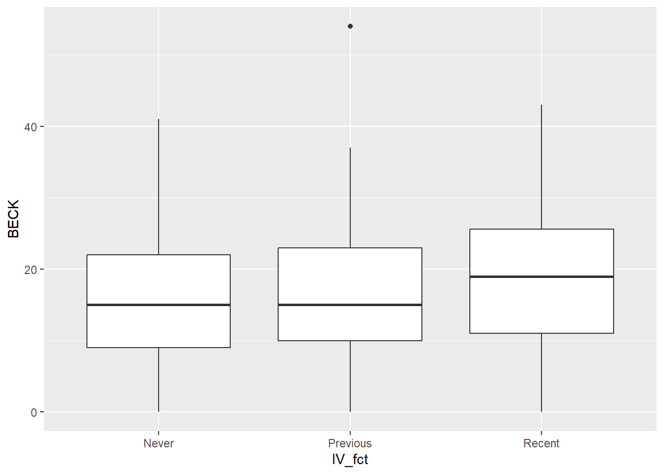
This boxplot shows that the distribution of depression scores is similar across the groups. There are some small differences, but it’s not clear if these differences are statistically significant.
We can get the overall mean of all Beck scores, sometimes called the “grand mean”.
If we use group_by, we can separate this out by IV group:
Exericse 3
We have to be careful about the term “grand mean”. In some contexts, the term “grand mean” refers to the mean of all scores in the response variable (17.36743 above). In other cases, the term refers to the mean of the three group means (the mean of 15.94996, 16.64201, and 18.99363).
First calculate the mean of the three group means above. (You can use R to do this if you want, or you can just use a calculator.) Explain mathematically why the overall mean 17.36743 is not the same as the mean of the three group means. What would have to be true of the sample for the overall mean to agree with the mean of the three group means? (Hint: think about the size of each of the three groups.)
Please write up your answer here.
22.5 The F distribution
To keep the exposition simple here, we’ll assume that the term “grand mean” refers to the overall mean of the response variable, 17.36743.
When assessing the differences among groups, there are two numbers that are important.
The first is called the “mean square between groups” (MSG). It measures how far away each group mean is away from the overall grand mean for the whole sample. For example, for those who never used IV drugs, their mean Beck score was 15.95. This is 1.42 points below the grand mean of 17.37. On the other hand, recent IV drug users had a mean Beck score of nearly 19. This is 1.63 points above the grand mean. MSG is calculated by taking these differences for each group, squaring them to make them positive, weighting them by the sizes of each group (larger groups should obviously count for more), and dividing by the “group degrees of freedom” \(df_{G} = k - 1\) where \(k\) is the number of groups. The idea is that MSG is a kind of “average variability” among the groups. In other words, how far away are the groups from the grand mean (and therefore, from each other)?
The second number of interest is the “mean square error” (MSE). It is a measure of variability within groups. In other words, it measures how far away data points are from their own group means. Even under the assumption of a null hypothesis that says all the groups should be the same, we still expect some variability. Its calculation also involves dividing by some degrees of freedom, but now it is \(df_{E} = n - k\).
All that is somewhat technical and complicated. We’ll leave it to the computer. The key insight comes from considering the ratio of \(MSG\) and \(MSE\). We will call this quantity F:
\[ F = \frac{MSG}{MSE}. \]
What can be said about this magical F? Under the assumption of the null hypothesis, we expect some variability among the groups, and we expect some variability within each group as well, but these two sources of variability should be about the same. In other words, \(MSG\) should be roughly equal to \(MSE\). Therefore, F ought to be close to 1.
We can simulate this using the infer package. Suppose that there were no difference in the mean BECK scores among the three groups. We can accomplish this by shuffling the IV labels, an idea we’ve seen several times before in this book. Permuting the IV values breaks any association that might have existed in the original data.
set.seed(420)
BECK_IV_test_sim <- uis2 %>%
  specify(response = BECK, explanatory = IV_fct) %>%
  hypothesize(null = "independence") %>%
  generate(reps = 1000, type = "permute") %>%
  calculate(stat = "F")
BECK_IV_test_sim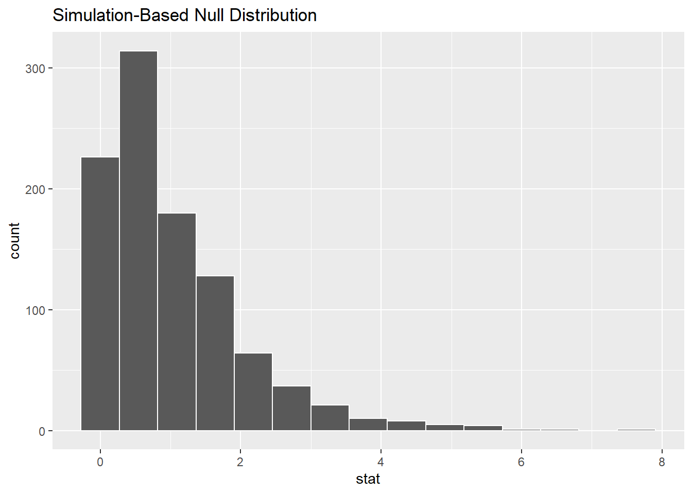
As explained earlier, the F scores are clustered around 1. They can never be smaller than zero. (The bar at zero is centered on zero, but no F score can be less than zero.) There are occasional F scores much larger than 1, but just by chance.
It’s not particularly interesting if F is less than one. That just means that the variability between groups is small and the variability of the data within each group is large. That doesn’t allow us to conclude that there is a difference among groups. However, if F is really large, that means that there is much more variability between the groups than there is within each group. Therefore, the groups are far apart and there is evidence of a difference among groups.
\(MSG\) and \(MSE\) are measures of variability, and that’s why this is called “Analysis of Variance”.
The F distribution is the correct sampling distribution model. Like a t model, there are infinitely many different F models because degrees of freedom are involved. But unlike a t model, the F model has two numbers called degrees of freedom, \(df_{G}\) and \(df_{E}\). Both of these numbers affect the precise shape of the F distribution.
For example, here is picture of a few different F models.
# Don't worry about the syntax here.
# You won't need to know how to do this on your own.
ggplot(data.frame(x = c(0, 5)), aes(x)) +
    stat_function(fun = df, args = list(df1 = 2, df2 = 5),
                  aes(color = "2, 5")) +
    stat_function(fun = df, args = list(df1 = 2, df2 = 50),
                  aes(color = "2, 50" )) +
    stat_function(fun = df, args = list(df1 = 10, df2 = 50),
                  aes(color = "10, 50")) +
    scale_color_manual(name = expression(paste(df[G], ", ", df[E])),
                       values = c("2, 5" = "red",
                                  "2, 50" = "blue",
                                  "10, 50" = "green"),
                       breaks =  c("2, 5", "2, 50", "10, 50"))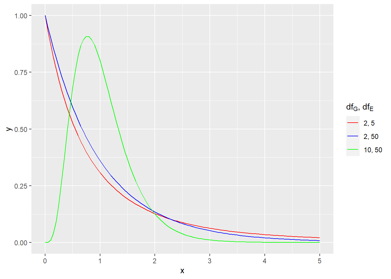
Here is the theoretical F distribution for our data:
BECK_IV_test <- uis2 %>%
  specify(response = BECK, explanatory = IV_fct) %>%
  hypothesize(null = "independence") %>%
  assume(distribution = "F")
BECK_IV_test
## An F distribution with 2 and 572 degrees of freedom.Exercise 4
Explain why there are 2 and 572 degrees of freedom. Which one is \(df_{G}\) and which one is \(df_{E}\)?
Please write up your answer here.
Here are the simulated values again, but with the theoretical F distribution superimposed for comparison.
## Warning: Check to make sure the conditions have been met for the theoretical
## method. {infer} currently does not check these for you.
## Warning: The dot-dot notation (`..density..`) was deprecated in ggplot2 3.4.0.
## ℹ Please use `after_stat(density)` instead.
## ℹ The deprecated feature was likely used in the infer package.
## Please report the issue at <https://github.com/tidymodels/infer/issues>.
## This warning is displayed once every 8 hours.
## Call `lifecycle::last_lifecycle_warnings()` to see where this warning was
## generated.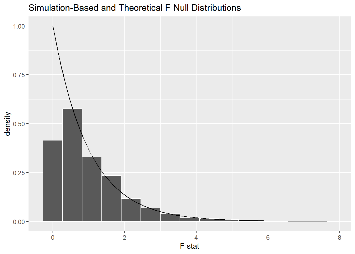
Other than the very left edge, the theoretical curve is a good fit to the simulated F scores.
22.6 Assumptions
What conditions can we check to justify the use of an F model for our sampling distribution? In addition to the typical “Random” and “10%” conditions that ensure independence, we also need to check the “Nearly normal” condition for each group, just like for the t tests. A new assumption is the “Constant variance” assumption, which says that each group should have the same variance in the population. This is impossible to check, although we can use our sample as a rough guide. If each group has about the same spread, that is some evidence that such an assumption might hold in the population as well. Also, ANOVA is pretty robust to this assumption, especially when the groups are close to the same size. Even when the group sizes are unequal (sometimes called “unbalanced”), some say the variances can be off by up to a factor of 3 and ANOVA will still work pretty well. So what we’re looking for here are gross violations, not minor ones.
Let’s go through the rubric with commentary.
22.7 Exploratory data analysis
22.7.1 Use data documentation (help files, code books, Google, etc.) to determine as much as possible about the data provenance and structure.
You should have researched this extensively in a previous exercise.
uis
glimpse(uis)## Rows: 575
## Columns: 18
## $ ID <dbl> 1, 2, 3, 4, 5, 6, 7, 8, 9, 10, 12, 13, 14, 15, 16, 17, 18, 19, …
## $ AGE <dbl> 39, 33, 33, 32, 24, 30, 39, 27, 40, 36, 38, 29, 32, 41, 31, 27,…
## $ BECK <dbl> 9.000, 34.000, 10.000, 20.000, 5.000, 32.550, 19.000, 10.000, 2…
## $ HC <dbl> 4, 4, 2, 4, 2, 3, 4, 4, 2, 2, 2, 3, 3, 1, 1, 2, 1, 4, 3, 2, 3, …
## $ IV <dbl> 3, 2, 3, 3, 1, 3, 3, 3, 3, 3, 3, 1, 3, 3, 3, 3, 3, 2, 1, 3, 1, …
## $ NDT <dbl> 1, 8, 3, 1, 5, 1, 34, 2, 3, 7, 8, 1, 2, 8, 1, 3, 6, 1, 15, 5, 1…
## $ RACE <dbl> 0, 0, 0, 0, 1, 0, 0, 0, 0, 0, 0, 0, 1, 0, 0, 0, 0, 0, 1, 0, 0, …
## $ TREAT <dbl> 1, 1, 1, 0, 1, 1, 1, 1, 1, 1, 1, 1, 1, 1, 1, 1, 1, 1, 1, 1, 0, …
## $ SITE <dbl> 0, 0, 0, 0, 0, 0, 0, 0, 0, 0, 0, 0, 0, 0, 0, 0, 0, 0, 0, 0, 0, …
## $ LEN.T <dbl> 123, 25, 7, 66, 173, 16, 179, 21, 176, 124, 176, 79, 182, 174, …
## $ TIME <dbl> 188, 26, 207, 144, 551, 32, 459, 22, 210, 184, 212, 87, 598, 26…
## $ CENSOR <dbl> 1, 1, 1, 1, 0, 1, 1, 1, 1, 1, 1, 1, 0, 1, 1, 1, 1, 1, 1, 1, 0, …
## $ Y <dbl> 5.236442, 3.258097, 5.332719, 4.969813, 6.311735, 3.465736, 6.1…
## $ ND1 <dbl> 5.0000000, 1.1111111, 2.5000000, 5.0000000, 1.6666667, 5.000000…
## $ ND2 <dbl> -8.0471896, -0.1170672, -2.2907268, -8.0471896, -0.8513760, -8.…
## $ LNDT <dbl> 0.6931472, 2.1972246, 1.3862944, 0.6931472, 1.7917595, 0.693147…
## $ FRAC <dbl> 0.68333333, 0.13888889, 0.03888889, 0.73333333, 0.96111111, 0.0…
## $ IV3 <dbl> 1, 0, 1, 1, 0, 1, 1, 1, 1, 1, 1, 0, 1, 1, 1, 1, 1, 0, 0, 1, 0, …22.7.2 Prepare the data for analysis. [Not always necessary.]
We need IV to be a factor variable.
# Although we've already done this above,
# we include it here again for completeness.
uis2 <- uis %>%
  mutate(IV_fct = factor(IV, levels = c(1, 2, 3),
                         labels = c("Never", "Previous", "Recent")))
uis2
glimpse(uis2)## Rows: 575
## Columns: 19
## $ ID <dbl> 1, 2, 3, 4, 5, 6, 7, 8, 9, 10, 12, 13, 14, 15, 16, 17, 18, 19, …
## $ AGE <dbl> 39, 33, 33, 32, 24, 30, 39, 27, 40, 36, 38, 29, 32, 41, 31, 27,…
## $ BECK <dbl> 9.000, 34.000, 10.000, 20.000, 5.000, 32.550, 19.000, 10.000, 2…
## $ HC <dbl> 4, 4, 2, 4, 2, 3, 4, 4, 2, 2, 2, 3, 3, 1, 1, 2, 1, 4, 3, 2, 3, …
## $ IV <dbl> 3, 2, 3, 3, 1, 3, 3, 3, 3, 3, 3, 1, 3, 3, 3, 3, 3, 2, 1, 3, 1, …
## $ NDT <dbl> 1, 8, 3, 1, 5, 1, 34, 2, 3, 7, 8, 1, 2, 8, 1, 3, 6, 1, 15, 5, 1…
## $ RACE <dbl> 0, 0, 0, 0, 1, 0, 0, 0, 0, 0, 0, 0, 1, 0, 0, 0, 0, 0, 1, 0, 0, …
## $ TREAT <dbl> 1, 1, 1, 0, 1, 1, 1, 1, 1, 1, 1, 1, 1, 1, 1, 1, 1, 1, 1, 1, 0, …
## $ SITE <dbl> 0, 0, 0, 0, 0, 0, 0, 0, 0, 0, 0, 0, 0, 0, 0, 0, 0, 0, 0, 0, 0, …
## $ LEN.T <dbl> 123, 25, 7, 66, 173, 16, 179, 21, 176, 124, 176, 79, 182, 174, …
## $ TIME <dbl> 188, 26, 207, 144, 551, 32, 459, 22, 210, 184, 212, 87, 598, 26…
## $ CENSOR <dbl> 1, 1, 1, 1, 0, 1, 1, 1, 1, 1, 1, 1, 0, 1, 1, 1, 1, 1, 1, 1, 0, …
## $ Y <dbl> 5.236442, 3.258097, 5.332719, 4.969813, 6.311735, 3.465736, 6.1…
## $ ND1 <dbl> 5.0000000, 1.1111111, 2.5000000, 5.0000000, 1.6666667, 5.000000…
## $ ND2 <dbl> -8.0471896, -0.1170672, -2.2907268, -8.0471896, -0.8513760, -8.…
## $ LNDT <dbl> 0.6931472, 2.1972246, 1.3862944, 0.6931472, 1.7917595, 0.693147…
## $ FRAC <dbl> 0.68333333, 0.13888889, 0.03888889, 0.73333333, 0.96111111, 0.0…
## $ IV3 <dbl> 1, 0, 1, 1, 0, 1, 1, 1, 1, 1, 1, 0, 1, 1, 1, 1, 1, 0, 0, 1, 0, …
## $ IV_fct <fct> Recent, Previous, Recent, Recent, Never, Recent, Recent, Recent…22.7.3 Make tables or plots to explore the data visually.
We should calculate group statistics:
tabyl(uis2, IV_fct) %>%
adorn_totals()Here are two graphs that are appropriate for one categorical and one numerical variable: a side-by-side boxplot and a stacked histogram.
ggplot(uis2, aes(y = BECK, x = IV_fct)) +
    geom_boxplot()
ggplot(uis2, aes(x = BECK)) +
    geom_histogram(binwidth = 5, boundary = 0) +
    facet_grid(IV_fct ~ .)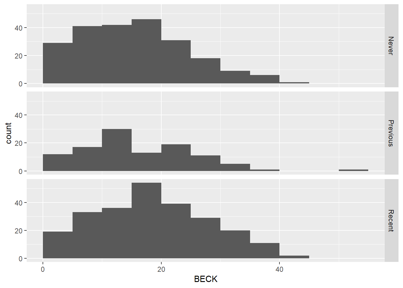
Both graphs show that the distribution of depression scores in each group is similar.
The distributions look reasonably normal, or perhaps a bit right skewed, but we can also check the QQ plots:
ggplot(uis2, aes(sample = BECK)) +
    geom_qq()  +
    geom_qq_line() +
    facet_grid(IV_fct ~ .)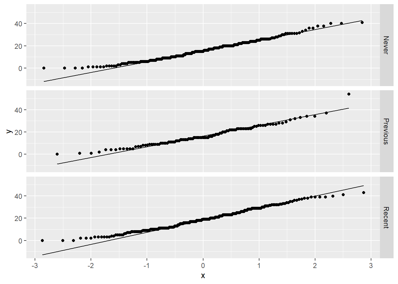
There is one mild outlier in the “Previous” group, but with sample sizes as large as we have in each group, it’s unlikely that this outlier will be influential. So we’ll just leave it in the data and not worry about it.
22.8 Hypotheses
22.8.1 Identify the sample (or samples) and a reasonable population (or populations) of interest.
The sample consists of people who participated in the UIS drug treatment study. Because the UIS studied the effects of residential treatment for drug abuse, the population is, presumably, all drug addicts.
22.8.2 Express the null and alternative hypotheses as contextually meaningful full sentences.
\(H_{0}:\) There is no difference in depression levels among those who have no history of IV drug use, those who have some previous IV drug use, and those who have recent IV drug use.
\(H_{A}:\) There is a difference in depression levels among those who have no history of IV drug use, those who have some previous IV drug use, and those who have recent IV drug use.
22.8.3 Express the null and alternative hypotheses in symbols (when possible).
\(H_{0}: \mu_{never} = \mu_{previous} = \mu_{recent}\)
There is no easy way to express the alternate hypothesis in symbols because any deviation in any of the categories can lead to rejection of the null. You can’t just say \(\mu_{never} \neq \mu_{previous} \neq \mu_{recent}\) because two of these categories might be the same and the third different and that would still be consistent with the alternative hypothesis.
So the only requirement here is to express the null in symbols.
22.9 Model
22.9.1 Identify the sampling distribution model.
We will use an F model with \(df_{G} = 2\) and \(df_{E} = 572\).
Commentary: Remember that
\[ df_{G} = k - 1 = 3 - 1 = 2, \]
(\(k\) is the number of groups, in this case, 3), and
\[ df_{E} = n - k = 575 - 3 = 572. \]
22.9.2 Check the relevant conditions to ensure that model assumptions are met.
- Random
- We have little information about how this sample was collected, so we have to hope it’s representative.
- 10%
- 575 is definitely less than 10% of all drug addicts.
- Nearly normal
- The earlier stacked histograms and QQ plots showed that each group is nearly normal. (There was one outlier in one group, but our sample sizes are quite large.)
- Constant variance
- The spread of data looks pretty consistent from group to group in the stacked histogram and side-by-side boxplot.
22.10 Mechanics
22.10.1 Compute the test statistic.
BECK_IV_F <- uis2 %>%
  specify(response = BECK, explanatory = IV_fct) %>%
  calculate(stat = "F")
BECK_IV_F
22.10.2 Report the test statistic in context (when possible).
The F score is 6.721405.
Commentary: F scores (much like chi-square values earlier in the course) are not particularly interpretable on their own, so there isn’t really any context we can provide. It’s only required that you report the F score in a full sentence.
22.10.3 Plot the null distribution.
BECK_IV_test <- uis2 %>%
  specify(response = BECK, explanatory = IV_fct) %>%
  hypothesize(null = "independence") %>%
  assume(distribution = "F")
BECK_IV_test
## An F distribution with 2 and 572 degrees of freedom.
BECK_IV_test %>%
  visualize() +
  shade_p_value(obs_stat = BECK_IV_F, direction = "greater")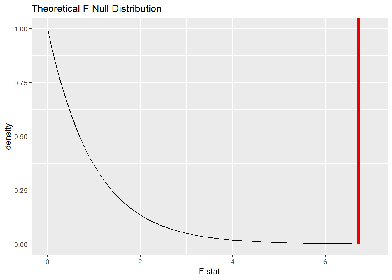
22.10.4 Calculate the P-value.
BECK_IV_P <- BECK_IV_test %>%
  get_p_value(obs_stat = BECK_IV_F, direction = "greater")
BECK_IV_P
Commentary: Note that this is, by definition, a one-sided test. Extreme values of F are the ones that are far away from 1, and only those values in the right tail are far from 1.
22.11 Conclusion
22.11.2 State (but do not overstate) a contextually meaningful conclusion.
There is sufficient evidence that there is a difference in depression levels among those who have no history of IV drug use, those who have some previous IV drug use, and those who have recent IV drug use.
22.11.3 Express reservations or uncertainty about the generalizability of the conclusion.
Our lack of uncertainty about the sample means we don’t know for sure if we can generalize to a larger population of drug users. We hope that the researchers would obtain a representative sample. Also, the study in question is from the 1990s, so we should not suppose that the conclusions are still true today.
22.11.4 Identify the possibility of either a Type I or Type II error and state what making such an error means in the context of the hypotheses.
If we’ve made a Type I error, that means that there really isn’t a difference among the three groups, but our sample is an unusual one that did detect a difference.
Exercise 5(a)
Everything we saw earlier in the exploratory data analysis pointed toward failing to reject the null. All three groups look very similar in all the plots, and the means are not all that far from each other. So why did we get such a tiny P-value and reject the null? In other words, what is it about our data that allows for small effects to be statistically significant?
Please write up your answer here.
Exercise 5(b)
If you were a psychologist working with drug addicts, would the statistical conclusion (rejecting the null and concluding that there was a difference among groups) be of clinical importance to you? In other words, if there is a difference, is it of practical significance and not just statistical significance?
Please write up your answer here.
There is no confidence interval for ANOVA. We are not hypothesizing about the value of any particular parameter, so there’s nothing to estimate with a confidence interval.
22.12 Your turn
Using the penguins data, determine if there is a difference in the average body masses among the three species represented in the data (Adelie, Chinstrap, and Gentoo).
There are two missing values of body mass, and as we saw earlier in the book, that does affect certain functions. To make it a little easier on you, here is some code to remove those missing values:
For this whole section, be sure to use penguins2.
The rubric outline is reproduced below. You may refer to the worked example above and modify it accordingly. Remember to strip out all the commentary. That is just exposition for your benefit in understanding the steps, but is not meant to form part of the formal inference process.
Another word of warning: the copy/paste process is not a substitute for your brain. You will often need to modify more than just the names of the data frames and variables to adapt the worked examples to your own work. Do not blindly copy and paste code without understanding what it does. And you should never copy and paste text. All the sentences and paragraphs you write are expressions of your own analysis. They must reflect your own understanding of the inferential process.
Also, so that your answers here don’t mess up the code chunks above, use new variable names everywhere.
Exploratory data analysis
Use data documentation (help files, code books, Google, etc.) to determine as much as possible about the data provenance and structure.
Please write up your answer here
# Add code here to print the data
# Add code here to glimpse the variablesHypotheses
Identify the sample (or samples) and a reasonable population (or populations) of interest.
Please write up your answer here.
Mechanics
Plot the null distribution.
# IF CONDUCTING A SIMULATION...
set.seed(1)
# Add code here to simulate the null distribution.
# Add code here to plot the null distribution.22.13 Bonus section: post-hoc analysis
Suppose our ANOVA test leads us to reject the null hypothesis. Then we have statistically significant evidence that there is some difference between the means of the various groups. However, ANOVA doesn’t tell us which groups are actually different – unsatisfying!
We could consider just doing a bunch of individual t-tests between each pair of groups. However, the problem with this approach is that it greatly increases the chances that we might commit a Type I error. (For an exploration of this problem, please see the following XKCD comic.)
Fortunately, there is a tool called post-hoc analysis that allows us to determine which groups differ from the others in a way that doesn’t inflate the Type I error rate.
There are several methods for conducting post-hoc analysis. You may have heard of the Bonferroni correction, in which the usual significance level is divided by the number of pairwise comparisons contemplated. Another method, and the one we’ll explore here, is called the Tukey Honestly-Significant-Difference test. The precise details of this test are a little outside the scope of this course, but here’s how it’s done in R.
We’ll start by using a different function, called aov, to conduct the ANOVA test. This function produces a slightly different format of outputs than we’re used to, but it produces all the same values as our other tools:
##              Df Sum Sq Mean Sq F value Pr(>F)
## IV_fct        2   1148   574.0   6.721 0.0013 **
## Residuals   572  48850    85.4
## ---
## Signif. codes:  0 '***' 0.001 '**' 0.01 '*' 0.05 '.' 0.1 ' ' 1
Notice in particular that the F score and the P-value are the same as we obtained using infer tools above.
Now that we have the result of the aov command stored in a new variable, we can feed it into the new command TukeyHSD:
TukeyHSD(BECK_IV_aov)## Tukey multiple comparisons of means
## 95% family-wise confidence level
##
## Fit: aov(formula = BECK ~ IV_fct, data = uis2)
##
## $IV_fct
## diff lwr upr p adj
## Previous-Never 0.692054 -1.8458349 3.229943 0.7976511
## Recent-Never 3.043674 1.0299195 5.057429 0.0012039
## Recent-Previous 2.351620 -0.1517446 4.854986 0.0707718Here’s how to read these results: Start by looking at the p adj column, which tells us adjusted p-values. Look for a p-value that is below the usual significance level \(\alpha = 0.05\). In our example, the second p-value is the only one that is small enough to reach significance.
Once you’ve located the significant p-values, read the row to determine which comparisons are significant. Here, the second row is the meaningful one: this is the comparison between the “Recent” group and the “Never” group.
The column labeled diff reports the difference between the means of the two groups; the order of subtraction is reported in the first column. Here, the difference in Beck depression scores is 3.043674, which is computed by subtracting the mean of the “Never” group from the mean of the “Recent” group.
As usual, we report our results in a contextually-meaningful sentence. Here’s our example:
Tukey’s HSD test reports that recent IV drug users have a Beck inventory score that is 3.043674 points higher than those who have never used IV drugs.
22.13.1 Your turn
Conduct a post-hoc analysis to determine which penguin species is heavier or lighter than the others.
# Add code here to produce the aov model

# Add code here to run Tukey's HSD test on the aov model
Report your results in a contextually-meaningful sentence:
Please write your answer here.
22.14 Conclusion
When analyzing a numerical response variable across three or more levels of a categorical predictor variable, ANOVA provides a way of comparing the variability of the response between the groups to the variability within the groups. When there is more variability between the groups than within the groups, this is evidence that the groups are truly different from one another (rather than simply arising from random sampling variability). The result of comparing the two sources of variability gives rise to the F distribution, which can be used to determine when the difference is more than one would expect from chance alone.
22.14.1 Preparing and submitting your assignment
- From the “Run” menu, select “Restart R and Run All Chunks”.
- Deal with any code errors that crop up. Repeat steps 1–-2 until there are no more code errors.
- Spell check your document by clicking the icon with “ABC” and a check mark.
- Hit the “Preview” button one last time to generate the final draft of the
.nb.htmlfile. - Proofread the HTML file carefully. If there are errors, go back and fix them, then repeat steps 1–5 again.
If you have completed this chapter as part of a statistics course, follow the directions you receive from your professor to submit your assignment.