21 Inference for two independent means
2.0
21.1 Introduction
If we have a numerical variable and a categorical variable with two categories, we can think of the numerical variable as response and the categorical variable as predictor. The idea is that the two categories sort your numerical data into two groups which can be compared. Assuming the two groups are independent of each other, we can use them as samples of two larger populations. This leads to inference to decide if the difference between the means of the two groups is statistically significant and then estimate the difference between the means of the two populations represented. The relevant hypothesis test is called a two-sample t test (or Welch’s t test, to be specific).
21.1.2 Download the R notebook file
Check the upper-right corner in RStudio to make sure you’re in your intro_stats project. Then click on the following link to download this chapter as an R notebook file (.Rmd).
Once the file is downloaded, move it to your project folder in RStudio and open it there.
21.2 Load packages
We load the standard tidyverse, janitor, and infer packages. We also use the MASS package for the birthwt data.
## ── Attaching core tidyverse packages ──────────────────────── tidyverse 2.0.0 ──
## ✔ dplyr     1.1.2     ✔ readr     2.1.4
## ✔ forcats   1.0.0     ✔ stringr   1.5.0
## ✔ ggplot2   3.4.2     ✔ tibble    3.2.1
## ✔ lubridate 1.9.2     ✔ tidyr     1.3.0
## ✔ purrr     1.0.2
## ── Conflicts ────────────────────────────────────────── tidyverse_conflicts() ──
## ✖ dplyr::filter() masks stats::filter()
## ✖ dplyr::lag()    masks stats::lag()
## ℹ Use the conflicted package (<http://conflicted.r-lib.org/>) to force all conflicts to become errors##
## Attaching package: 'janitor'
##
## The following objects are masked from 'package:stats':
##
## chisq.test, fisher.test##
## Attaching package: 'MASS'
##
## The following object is masked from 'package:dplyr':
##
## select21.3 Research question
Recall the birthwt data that was collected at Baystate Medical Center, Springfield, Mass during 1986. In a previous chapter, we measured low birth weight babies using a categorical variable that served as an indicator for low birth weight.
Exercise 1
How was it determined if a baby was considered “low birth weight” for purposes of constructing the variable low? Use the help file to find out.
Please write up your answer here.
We have the actual birth weight of the babies in this data. So, rather than using a coarse classification into a binary “yes or no” variable, why not use the full precision of the birth weight measured in grams? This is a very precisely measured numerical variable.
We’d like to compare mean birth weights among two groups: women who smoked during pregnancy, and women who didn’t.
21.4 Data preparation
The actual mean weights in each sample (the smoking women and the nonsmoking women) can be found using a group_by and summarise pipeline:
Note that 0 means “nonsmoker” and 1 means “smoker”. Looks like We need to address the fact the smoke variable is recorded as a numerical variable instead of a categorical variable. Here is birthwt2 that we will use from here on out:
birthwt2 <- birthwt %>%
    mutate(smoke_fct = factor(smoke, levels = c(0, 1), labels = c("Nonsmoker", "Smoker")))
birthwt2
glimpse(birthwt2)## Rows: 189
## Columns: 11
## $ low <int> 0, 0, 0, 0, 0, 0, 0, 0, 0, 0, 0, 0, 0, 0, 0, 0, 0, 0, 0, 0, …
## $ age <int> 19, 33, 20, 21, 18, 21, 22, 17, 29, 26, 19, 19, 22, 30, 18, …
## $ lwt <int> 182, 155, 105, 108, 107, 124, 118, 103, 123, 113, 95, 150, 9…
## $ race <int> 2, 3, 1, 1, 1, 3, 1, 3, 1, 1, 3, 3, 3, 3, 1, 1, 2, 1, 3, 1, …
## $ smoke <int> 0, 0, 1, 1, 1, 0, 0, 0, 1, 1, 0, 0, 0, 0, 1, 1, 0, 1, 0, 1, …
## $ ptl <int> 0, 0, 0, 0, 0, 0, 0, 0, 0, 0, 0, 0, 0, 1, 0, 0, 0, 0, 0, 0, …
## $ ht <int> 0, 0, 0, 0, 0, 0, 0, 0, 0, 0, 0, 0, 1, 0, 0, 0, 0, 0, 0, 0, …
## $ ui <int> 1, 0, 0, 1, 1, 0, 0, 0, 0, 0, 0, 0, 0, 1, 0, 0, 0, 0, 1, 0, …
## $ ftv <int> 0, 3, 1, 2, 0, 0, 1, 1, 1, 0, 0, 1, 0, 2, 0, 0, 0, 3, 0, 1, …
## $ bwt <int> 2523, 2551, 2557, 2594, 2600, 2622, 2637, 2637, 2663, 2665, …
## $ smoke_fct <fct> Nonsmoker, Nonsmoker, Smoker, Smoker, Smoker, Nonsmoker, Non…The difference between the means is now calculated using infer tools. We will store the result as obs_diff for “observed difference”.
obs_diff <- birthwt2 %>%
  specify(response = bwt, explanatory = smoke_fct) %>%
  calculate(stat = "diff in means", order = c("Nonsmoker", "Smoker"))
obs_diff
Exercise 2
What would happen if we used order = c("Smoker", "Nonsmoker") instead? Why might we have a slight preference for order = c("Nonsmoker", "Smoker")?
Please write up your answer here.
Note that it will not actually make a difference to the inferential process in which order we subtract. However, we do have to be consistent to use the same order throughout. When interpreting the test statistic, effect size, and confidence interval, we will need to pay attention to the order of subtraction to make sure we are interpreting our results correctly.
21.5 Every day I’m shuffling
Whenever there are two groups, the obvious null hypothesis is that there is no difference between them.
Consider the smoke variable. If there were truly no difference in mean birth weights between women who smoked and women who didn’t, then it shouldn’t matter if we know the smoking status or not. It becomes irrelevant under the assumption of the null.
We can simulate this assumption by shuffling the list of smoking status. More concretely, we can randomly assign a smoking status label to each mother and then calculate the average birth weight in each group. Since the smoking labels are random, there’s no reason to expect a difference between the two average weights other than random fluctuations due to sampling variability.
For example, here is the actual smoking status of the women:
birthwt2$smoke_fct## [1] Nonsmoker Nonsmoker Smoker Smoker Smoker Nonsmoker Nonsmoker
## [8] Nonsmoker Smoker Smoker Nonsmoker Nonsmoker Nonsmoker Nonsmoker
## [15] Smoker Smoker Nonsmoker Smoker Nonsmoker Smoker Nonsmoker
## [22] Nonsmoker Nonsmoker Nonsmoker Nonsmoker Nonsmoker Smoker Nonsmoker
## [29] Smoker Nonsmoker Nonsmoker Smoker Smoker Nonsmoker Nonsmoker
## [36] Smoker Smoker Smoker Smoker Smoker Smoker Nonsmoker
## [43] Nonsmoker Nonsmoker Smoker Smoker Nonsmoker Nonsmoker Nonsmoker
## [50] Smoker Nonsmoker Nonsmoker Smoker Smoker Nonsmoker Nonsmoker
## [57] Smoker Nonsmoker Nonsmoker Nonsmoker Nonsmoker Nonsmoker Nonsmoker
## [64] Nonsmoker Smoker Nonsmoker Nonsmoker Smoker Nonsmoker Nonsmoker
## [71] Smoker Smoker Smoker Nonsmoker Smoker Nonsmoker Nonsmoker
## [78] Smoker Smoker Nonsmoker Nonsmoker Nonsmoker Nonsmoker Nonsmoker
## [85] Nonsmoker Smoker Nonsmoker Nonsmoker Nonsmoker Nonsmoker Nonsmoker
## [92] Nonsmoker Smoker Smoker Smoker Nonsmoker Nonsmoker Smoker
## [99] Smoker Nonsmoker Nonsmoker Smoker Nonsmoker Nonsmoker Nonsmoker
## [106] Nonsmoker Nonsmoker Nonsmoker Smoker Nonsmoker Nonsmoker Nonsmoker
## [113] Smoker Nonsmoker Smoker Nonsmoker Nonsmoker Nonsmoker Nonsmoker
## [120] Nonsmoker Nonsmoker Nonsmoker Nonsmoker Nonsmoker Nonsmoker Nonsmoker
## [127] Nonsmoker Smoker Nonsmoker Nonsmoker Smoker Nonsmoker Smoker
## [134] Nonsmoker Nonsmoker Nonsmoker Nonsmoker Nonsmoker Nonsmoker Smoker
## [141] Smoker Smoker Nonsmoker Nonsmoker Smoker Smoker Nonsmoker
## [148] Smoker Nonsmoker Nonsmoker Nonsmoker Nonsmoker Smoker Smoker
## [155] Nonsmoker Smoker Smoker Smoker Nonsmoker Smoker Smoker
## [162] Nonsmoker Nonsmoker Nonsmoker Smoker Smoker Nonsmoker Nonsmoker
## [169] Smoker Nonsmoker Smoker Smoker Smoker Nonsmoker Nonsmoker
## [176] Smoker Smoker Smoker Smoker Nonsmoker Nonsmoker Nonsmoker
## [183] Smoker Smoker Smoker Nonsmoker Smoker Nonsmoker Smoker
## Levels: Nonsmoker SmokerBut we’re going to use values that have been randomly shuffled, like this one, for example:
##   [1] Nonsmoker Smoker    Nonsmoker Nonsmoker Smoker    Nonsmoker Smoker
##   [8] Nonsmoker Smoker    Nonsmoker Nonsmoker Smoker    Smoker    Nonsmoker
##  [15] Nonsmoker Nonsmoker Nonsmoker Smoker    Smoker    Nonsmoker Nonsmoker
##  [22] Nonsmoker Smoker    Nonsmoker Nonsmoker Nonsmoker Nonsmoker Smoker
##  [29] Nonsmoker Nonsmoker Nonsmoker Nonsmoker Smoker    Smoker    Nonsmoker
##  [36] Smoker    Smoker    Smoker    Nonsmoker Nonsmoker Nonsmoker Nonsmoker
##  [43] Nonsmoker Nonsmoker Nonsmoker Smoker    Nonsmoker Nonsmoker Nonsmoker
##  [50] Smoker    Nonsmoker Nonsmoker Smoker    Nonsmoker Smoker    Nonsmoker
##  [57] Nonsmoker Nonsmoker Smoker    Nonsmoker Nonsmoker Smoker    Smoker
##  [64] Nonsmoker Nonsmoker Smoker    Nonsmoker Nonsmoker Smoker    Nonsmoker
##  [71] Nonsmoker Nonsmoker Nonsmoker Smoker    Nonsmoker Nonsmoker Smoker
##  [78] Smoker    Smoker    Smoker    Smoker    Smoker    Smoker    Nonsmoker
##  [85] Smoker    Nonsmoker Smoker    Smoker    Smoker    Nonsmoker Nonsmoker
##  [92] Nonsmoker Nonsmoker Smoker    Smoker    Nonsmoker Nonsmoker Smoker
##  [99] Smoker    Nonsmoker Nonsmoker Smoker    Nonsmoker Smoker    Nonsmoker
## [106] Nonsmoker Nonsmoker Smoker    Nonsmoker Smoker    Smoker    Smoker
## [113] Nonsmoker Smoker    Smoker    Nonsmoker Nonsmoker Smoker    Nonsmoker
## [120] Nonsmoker Nonsmoker Nonsmoker Smoker    Smoker    Smoker    Smoker
## [127] Nonsmoker Nonsmoker Nonsmoker Smoker    Smoker    Smoker    Nonsmoker
## [134] Nonsmoker Nonsmoker Smoker    Nonsmoker Nonsmoker Nonsmoker Smoker
## [141] Nonsmoker Nonsmoker Smoker    Nonsmoker Nonsmoker Smoker    Nonsmoker
## [148] Smoker    Nonsmoker Nonsmoker Smoker    Nonsmoker Smoker    Smoker
## [155] Smoker    Nonsmoker Nonsmoker Nonsmoker Smoker    Smoker    Nonsmoker
## [162] Nonsmoker Nonsmoker Nonsmoker Nonsmoker Nonsmoker Nonsmoker Nonsmoker
## [169] Nonsmoker Smoker    Smoker    Nonsmoker Smoker    Nonsmoker Nonsmoker
## [176] Nonsmoker Smoker    Smoker    Nonsmoker Nonsmoker Nonsmoker Nonsmoker
## [183] Smoker    Nonsmoker Nonsmoker Nonsmoker Smoker    Nonsmoker Nonsmoker
## Levels: Nonsmoker Smoker
The infer package will perform this random shuffling over and over again. Given the now arbitrary labels of “Nonsmoker” and “Smoker” (which are meaningless because each women was assigned to one of these labels randomly with no regard to her actual smoking status), infer will calculate the mean birth weights among the first group of women (labeled “Nonsmokers” but not really consisting of all nonsmokers) and the second group of women (labeled “Smokers” but not really consisting of all smokers). Finally infer will compute the difference between those two means. And it will do this process 1000 times.
set.seed(1729)
bwt_smoke_test <- birthwt2 %>%
  specify(response = bwt, explanatory = smoke_fct) %>%
  hypothesize(null = "independence") %>%
  generate(reps = 1000, type = "permute") %>%
  calculate(stat = "diff in means", order = c("Nonsmoker", "Smoker"))
bwt_smoke_test
Exercise 3
Before we graph these simulated values, what do you guess will be the mean value? Keep in mind that we have computed differences in the mean birth weights between two groups of women. But because we have shuffled the smoking labels randomly, we aren’t really calculating the difference in mean birth weights of nonsmokers vs smokers. We’re just computing the difference in mean birth weights of randomly assigned groups of women.
Please write up your answer here.
Here’s the visualization:
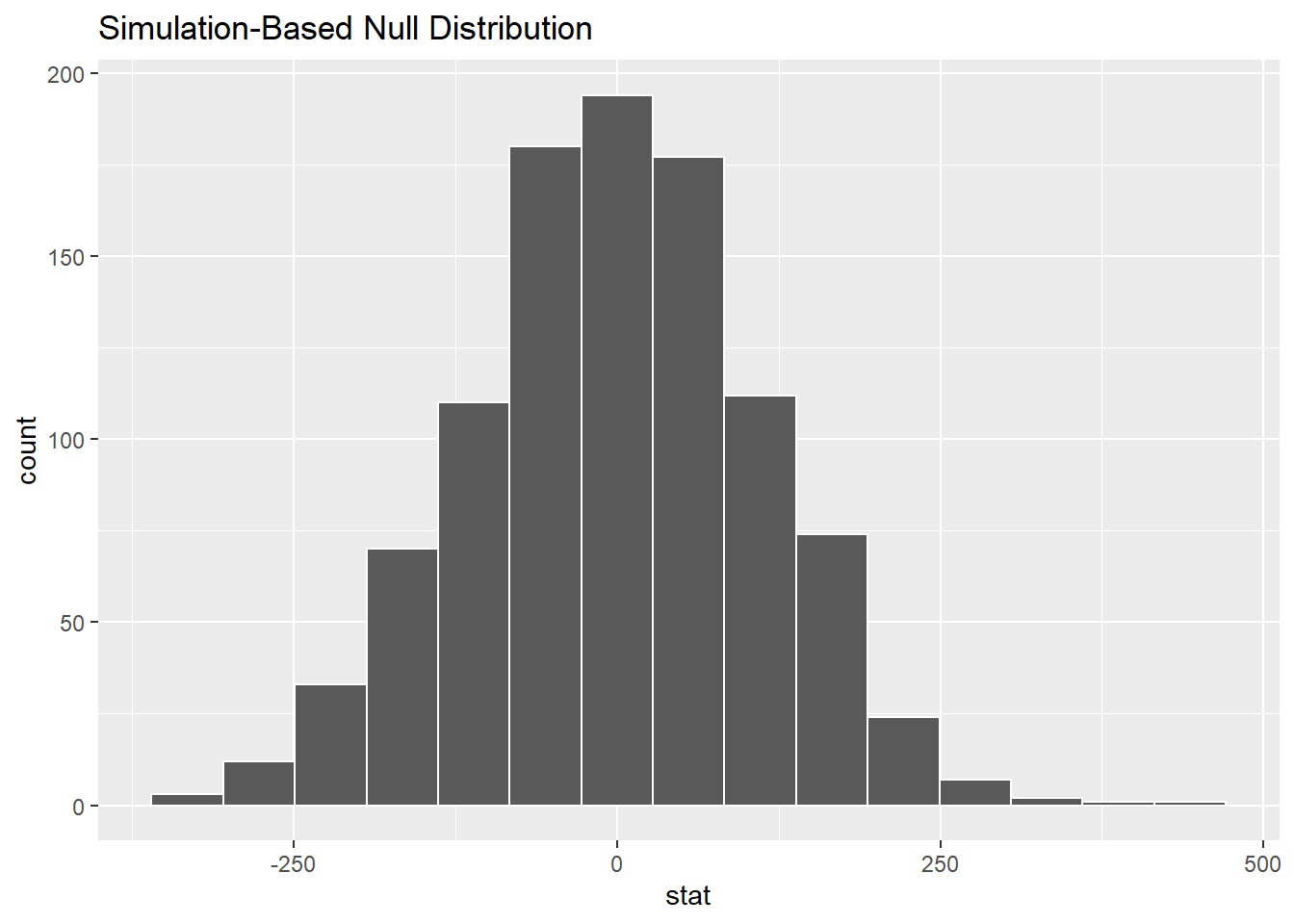
No surprise that this histogram looks nearly normal, centered at zero: the simulation is working under the assumption of the null hypothesis of no difference between the groups.
Here is the same plot but including our sample difference:
bwt_smoke_test %>%
visualize() +
shade_p_value(obs_stat = obs_diff, direction = "two_sided")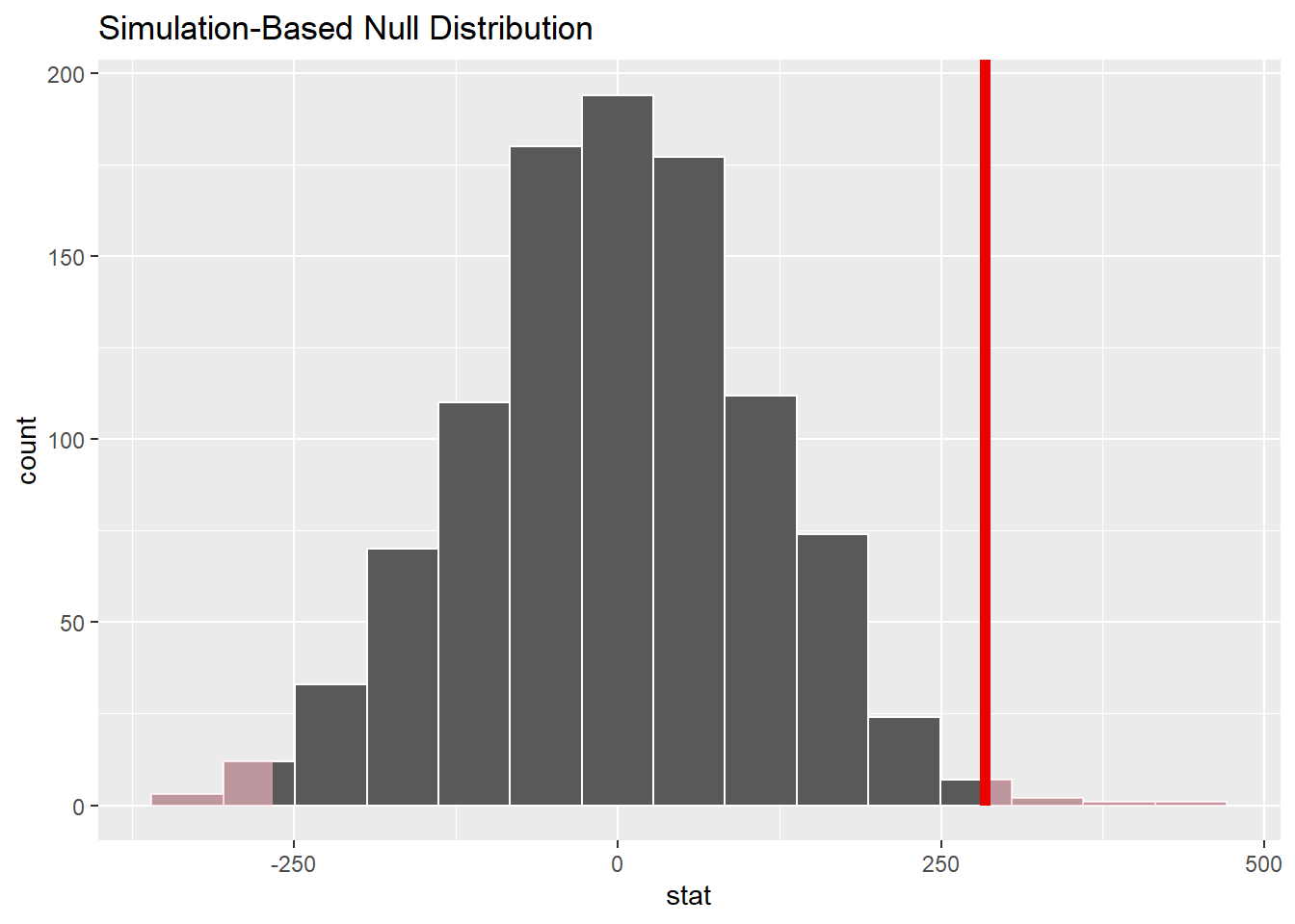
Our observed difference (from the sampled data) is quite far out into the tail of this simulated sampling distribution, so it appears that our actual data would be somewhat unlikely due to pure chance alone if the null hypothesis were true.
We can even find a P-value by calculating how many of our sampled values are as extreme or more extreme than the observed data difference.
bwt_smoke_test %>%
    get_p_value(obs_stat = obs_diff, direction = "two-sided")
Indeed, this is a small P-value.
21.6 The sampling distribution model
In the previous section, we simulated the sampling distribution under the assumption of a null hypothesis of no difference between the groups. It certainly looked like a normal model, but which normal model? The center is obviously zero, but what about the standard deviation?
Let’s assume that both groups come from populations that are normally distributed with normal models \(N(\mu_{1}, \sigma_{1})\) and \(N(\mu_{2}, \sigma_{2})\). If we take samples of size \(n_{1}\) from group 1 and \(n_{2}\) from group 2, some fancy math shows that the distribution of the differences between sample means is
\[ N\left(\mu_{1} - \mu_{2}, \sqrt{\frac{\sigma_{1}^{2}}{n_{1}} + \frac{\sigma_{2}^{2}}{n_{2}}}\right). \]
Under the assumption of the null, the difference of the means is zero (\(\mu_{1} - \mu_{2} = 0\)). Unfortunately, though, we make no assumption on the standard deviations. It should be clear that the only solution is to substitute the sample standard deviations \(s_{1}\) and \(s_{2}\) for the population standard deviations \(\sigma_{1}\) and \(\sigma_{2}\).21
\[ SE = \sqrt{\frac{s_{1}^{2}}{n_{1}} + \frac{s_{2}^{2}}{n_{2}}}. \]
However, \(s_{1}\) and \(s_{2}\) are not perfect estimates of \(\sigma_{1}\) and \(\sigma_{2}\); they are subject to sampling variability too. This extra variability means that a normal model is no longer appropriate as the sampling distribution model.
In the one-sample case, a Student t model with \(df = n - 1\) was the right choice. In the two-sample case, we don’t know the right answer. And I don’t mean that we haven’t learned it yet in our stats class. I mean, statisticians have not found a formula for the correct sampling distribution. It is a famous unsolved problem, called the Behrens-Fisher problem.
Several researchers have proposed solutions that are “close” though. One compelling one is called “Welch’s t test”. Welch showed that even though it’s not quite right, a Student t model is very close as long as you pick the degrees of freedom carefully. Unfortunately, the way to compute the right degrees of freedom is crazy complicated. Fortunately, R is good at crazy complicated computations.
Let’s go through the full rubric.
21.7 Exploratory data analysis
21.7.1 Use data documentation (help files, code books, Google, etc.) to determine as much as possible about the data provenance and structure.
Type birthwt at the Console to read the help file. We have the same concerns about the lack of details as we did in Chapter 16.
birthwt
glimpse(birthwt)## Rows: 189
## Columns: 10
## $ low <int> 0, 0, 0, 0, 0, 0, 0, 0, 0, 0, 0, 0, 0, 0, 0, 0, 0, 0, 0, 0, 0, 0…
## $ age <int> 19, 33, 20, 21, 18, 21, 22, 17, 29, 26, 19, 19, 22, 30, 18, 18, …
## $ lwt <int> 182, 155, 105, 108, 107, 124, 118, 103, 123, 113, 95, 150, 95, 1…
## $ race <int> 2, 3, 1, 1, 1, 3, 1, 3, 1, 1, 3, 3, 3, 3, 1, 1, 2, 1, 3, 1, 3, 1…
## $ smoke <int> 0, 0, 1, 1, 1, 0, 0, 0, 1, 1, 0, 0, 0, 0, 1, 1, 0, 1, 0, 1, 0, 0…
## $ ptl <int> 0, 0, 0, 0, 0, 0, 0, 0, 0, 0, 0, 0, 0, 1, 0, 0, 0, 0, 0, 0, 0, 0…
## $ ht <int> 0, 0, 0, 0, 0, 0, 0, 0, 0, 0, 0, 0, 1, 0, 0, 0, 0, 0, 0, 0, 0, 0…
## $ ui <int> 1, 0, 0, 1, 1, 0, 0, 0, 0, 0, 0, 0, 0, 1, 0, 0, 0, 0, 1, 0, 0, 1…
## $ ftv <int> 0, 3, 1, 2, 0, 0, 1, 1, 1, 0, 0, 1, 0, 2, 0, 0, 0, 3, 0, 1, 2, 3…
## $ bwt <int> 2523, 2551, 2557, 2594, 2600, 2622, 2637, 2637, 2663, 2665, 2722…21.7.2 Prepare the data for analysis.
We need to be sure smoke is a factor variable, so we create the new tibble birthwt2 with the mutated variable smoke_fct.
birthwt2 <- birthwt %>%
    mutate(smoke_fct = factor(smoke, levels = c(0, 1), labels = c("Nonsmoker", "Smoker")))
birthwt2
glimpse(birthwt2)## Rows: 189
## Columns: 11
## $ low <int> 0, 0, 0, 0, 0, 0, 0, 0, 0, 0, 0, 0, 0, 0, 0, 0, 0, 0, 0, 0, …
## $ age <int> 19, 33, 20, 21, 18, 21, 22, 17, 29, 26, 19, 19, 22, 30, 18, …
## $ lwt <int> 182, 155, 105, 108, 107, 124, 118, 103, 123, 113, 95, 150, 9…
## $ race <int> 2, 3, 1, 1, 1, 3, 1, 3, 1, 1, 3, 3, 3, 3, 1, 1, 2, 1, 3, 1, …
## $ smoke <int> 0, 0, 1, 1, 1, 0, 0, 0, 1, 1, 0, 0, 0, 0, 1, 1, 0, 1, 0, 1, …
## $ ptl <int> 0, 0, 0, 0, 0, 0, 0, 0, 0, 0, 0, 0, 0, 1, 0, 0, 0, 0, 0, 0, …
## $ ht <int> 0, 0, 0, 0, 0, 0, 0, 0, 0, 0, 0, 0, 1, 0, 0, 0, 0, 0, 0, 0, …
## $ ui <int> 1, 0, 0, 1, 1, 0, 0, 0, 0, 0, 0, 0, 0, 1, 0, 0, 0, 0, 1, 0, …
## $ ftv <int> 0, 3, 1, 2, 0, 0, 1, 1, 1, 0, 0, 1, 0, 2, 0, 0, 0, 3, 0, 1, …
## $ bwt <int> 2523, 2551, 2557, 2594, 2600, 2622, 2637, 2637, 2663, 2665, …
## $ smoke_fct <fct> Nonsmoker, Nonsmoker, Smoker, Smoker, Smoker, Nonsmoker, Non…21.7.3 Make tables or plots to explore the data visually.
How many women are in each group?
tabyl(birthwt2, smoke_fct) %>%
  adorn_totals()
With a numerical response variable and a categorical predictor variable, there are two useful plots: a side-by-side boxplot and a stacked histogram.
ggplot(birthwt2, aes(y = bwt, x = smoke_fct)) +
    geom_boxplot()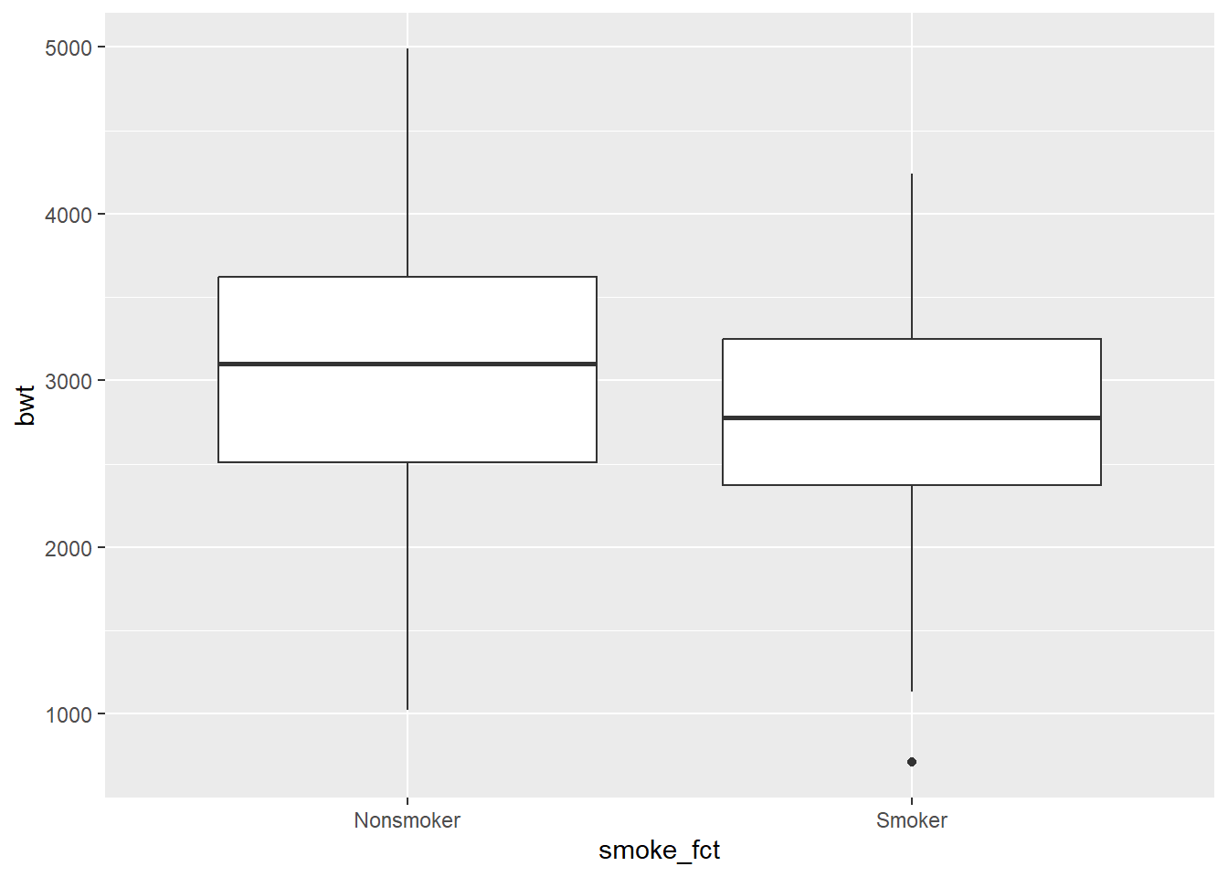
ggplot(birthwt2, aes(x = bwt)) +
    geom_histogram(binwidth = 250, boundary = 0) +
    facet_grid(smoke_fct ~ .)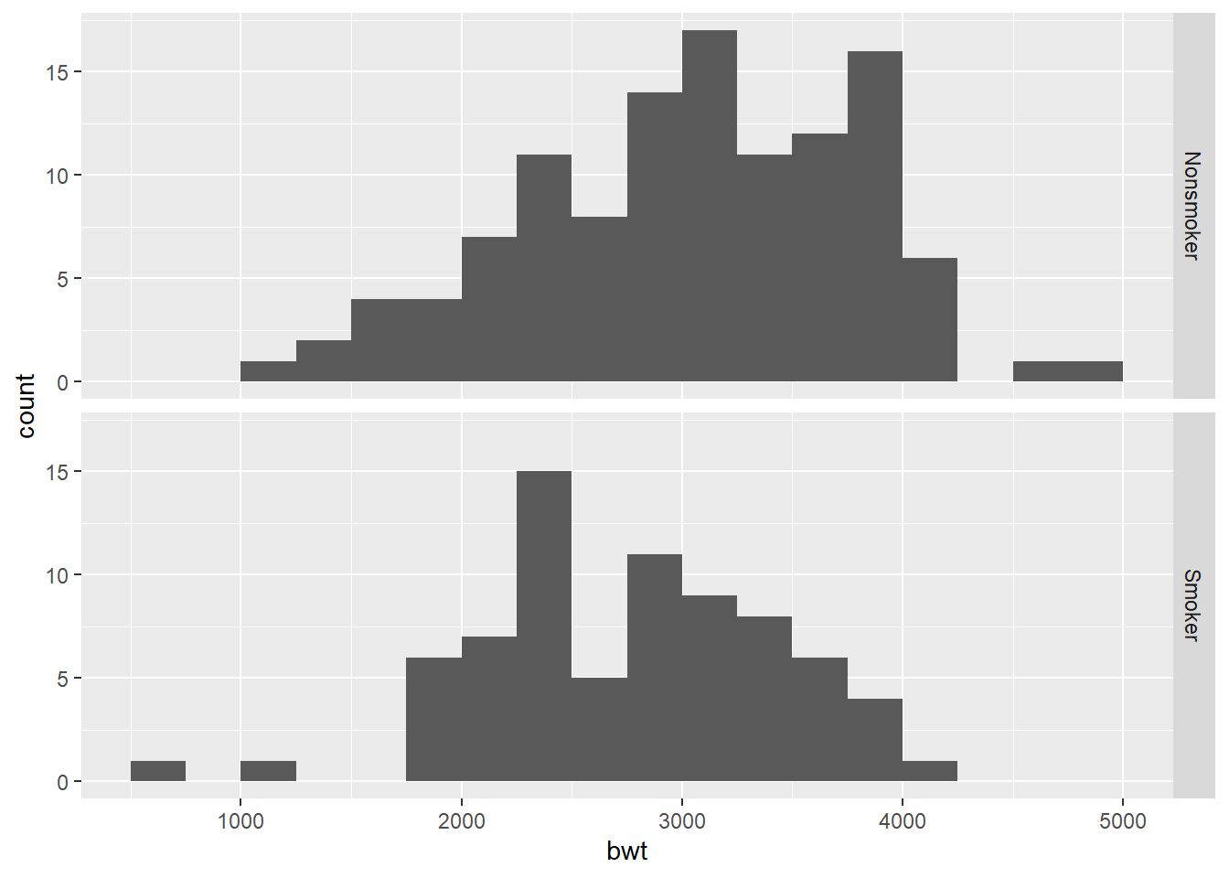
The histograms for both groups look sort of normal, but the nonsmoker group may be a little left skewed and the smoker group may have some low outliers. Here are the QQ plots to give us another way to ascertain normality of the data.
ggplot(birthwt2, aes(sample = bwt)) +
    geom_qq() +
    geom_qq_line() +
    facet_grid(smoke_fct ~ .)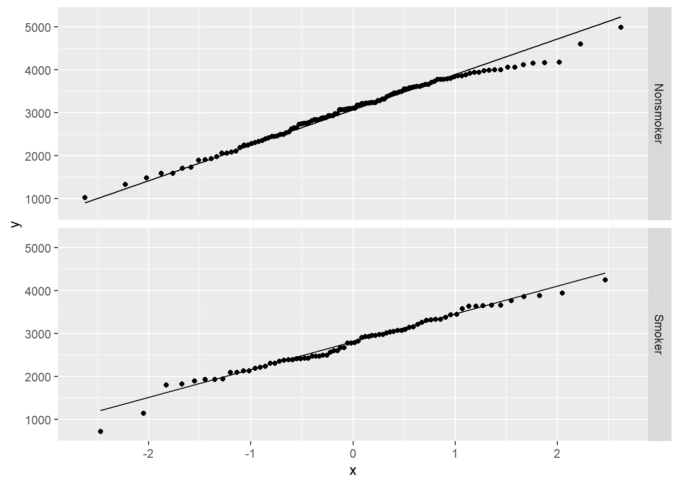
There’s a little deviation from normality, but nothing too crazy.
Commentary: The boxplots and histograms show why statistical inference is so important. It’s clear that there is some difference between the two groups, but it’s not obvious if that difference will turn out to be statistically significant. There appears to be a lot of variability in both groups, and both groups have a fair number of lighter and heavier babies.
21.8 Hypotheses
21.8.1 Identify the sample (or samples) and a reasonable population (or populations) of interest.
The samples consist of 115 nonsmoking mothers and 74 smoking mothers. The populations are those women who do not smoke during pregnancy and those women who do smoke during pregnancy.
21.8.2 Express the null and alternative hypotheses as contextually meaningful full sentences.
\(H_{0}:\) There is no difference in the birth weight of babies born to mothers who do not smoke versus mothers who do smoke.
\(H_{A}:\) There is a difference in the birth weight of babies born to mothers who do not smoke versus mothers who do smoke.
21.8.3 Express the null and alternative hypotheses in symbols (when possible).
\(H_{0}: \mu_{Nonsmoker} - \mu_{Smoker} = 0\)
\(H_{A}: \mu_{Nonsmoker} - \mu_{Smoker} \neq 0\)
Commentary: As mentioned before, the order in which you subtract will not change the inference, but it will affect your interpretation of the results. Also, once you’ve chosen a direction to subtract, be consistent about that choice throughout the rubric.
21.9 Model
21.9.1 Identify the sampling distribution model.
We use a t model with the number of degrees of freedom to be determined.
Commentary: For Welch’s t test, the degrees of freedom won’t usually be a whole number. Be sure you understand that the formula is no longer \(df = n - 1\). That doesn’t even make any sense as there isn’t a single \(n\) in a two-sample test. The infer package will tell us how many degrees of freedom to use later in the Mechanics section.
21.9.2 Check the relevant conditions to ensure that model assumptions are met.
- Random (for both groups)
- We have very little information about these women. We hope that the 115 nonsmoking mothers at this hospital are representative of other nonsmoking mothers, at least in that region at that time. And same for the 74 smoking mothers.
- 10% (for both groups)
- 115 is less than 10% of all nonsmoking mothers and 74 is less than 10% of all smoking mothers.
- Nearly normal (for both groups)
- Since the sample sizes are more than 30 in each group, we meet the condition.
21.10 Mechanics
21.10.1 Compute the test statistic.
obs_diff <- birthwt2 %>%
  specify(response = bwt, explanatory = smoke_fct) %>%
  calculate(stat = "diff in means", order = c("Nonsmoker", "Smoker"))
obs_diff
obs_diff_t <- birthwt2 %>%
  specify(response = bwt, explanatory = smoke_fct) %>%
  calculate(stat = "t", order = c("Nonsmoker", "Smoker"))
obs_diff_t
21.10.2 Report the test statistic in context (when possible).
The difference in the mean birth weight of babies born to nonsmoking mothers and smoking mothers is 283.7767333 grams. This was obtained by subtracting nonsmoking mothers minus smoking mothers. In other words, the fact that this is positive indicates that nonsmoking mothers had heavier babies, on average, than smoking mothers.
The t score is 2.7298857. The sample difference in birth weights is about 2.7 standard errors higher than the null value of zero.
Commentary: Remember that whenever you are computing the difference between two quantities, you must indicate the direction of that difference you so your reader knows how to interpret the value, whether it is positive or negative.
21.10.3 Plot the null distribution.
bwt_smoke_test_t <- birthwt2 %>%
  specify(response = bwt, explanatory = smoke_fct) %>%
  hypothesise(null = "independence") %>%
  assume("t")
bwt_smoke_test_t
## A T distribution with 170 degrees of freedom.
bwt_smoke_test_t %>%
  visualize() +
  shade_p_value(obs_stat = obs_diff_t, direction = "two-sided")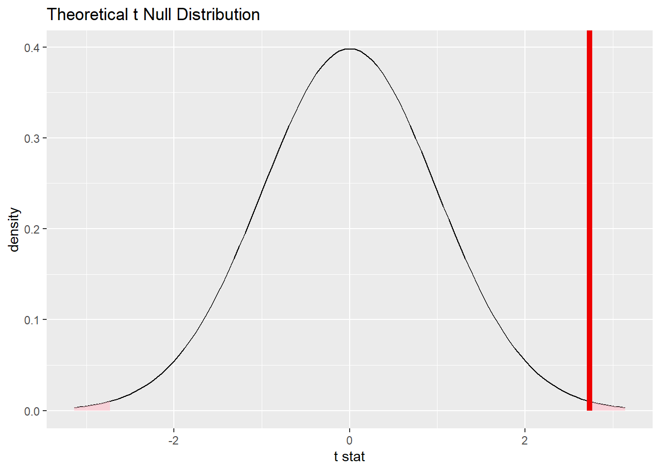
Commentary: We use the name bwt_smoke_test_t (using the assumption of a Student t model) as a new variable name so that it doesn’t overwrite the variable bwt_smoke_test we performed earlier as a permutation test (the one with the shuffling). This results of using bwt_smoke_test versus bwt_smoke_test_t will be very similar.
Note that the infer output tells us there are 170 degrees of freedom. (It turns out to be 170.1.) Note that this number is the result of a complicated formula, and it’s not just a simple function of the sample sizes 115 and 74.
Finally, note that the alternative hypothesis indicated a two-sided test, so we need to specify a “two-sided” P-value in the shade_p_value command.
21.10.4 Calculate the P-value.
bwt_smoke_p <- bwt_smoke_test_t %>%
  get_p_value(obs_stat = obs_diff_t, direction = "two-sided")
bwt_smoke_p21.11 Conclusion
21.11.2 State (but do not overstate) a contextually meaningful conclusion.
We have sufficient evidence that there is a difference in the mean birth weight of babies born to mothers who do not smoke versus mothers who do smoke.
21.11.3 Express reservations or uncertainty about the generalizability of the conclusion.
As when we looked at this data before, our uncertainly about the data provenance means that we don’t know if the difference observed in these samples at this one hospital at this one time are generalizable to larger populations. Also keep in mind that this data is observational, so we cannot draw any causal conclusion about the “effect” of smoking on birth weight.
21.11.4 Identify the possibility of either a Type I or Type II error and state what making such an error means in the context of the hypotheses.
If we’ve made a Type I error, then that means that there might be no difference in the birth weights of babies from nonsmoking versus smoking mothers, but we got some unusual samples that showed a difference.
21.12 Confidence interval
21.12.1 Check the relevant conditions to ensure that model assumptions are met.
There are no additional conditions to check.
21.12.2 Calculate the confidence interval.
bwt_smoke_ci <- bwt_smoke_test_t %>%
  get_confidence_interval(point_estimate = obs_diff, level = 0.95)
bwt_smoke_ci
Commentary: Pay close attention to when we use obs_diff and obs_diff_t. In the hypothesis test, we assumed a t distribution for the null and so we have to use the t score obs_diff_t to shade the P-value. However, for a confidence interval, we are building the interval centered on our sample difference obs_diff.
21.12.3 State (but do not overstate) a contextually meaningful interpretation.
We are 95% confident that the true difference in birth weight between nonsmoking and smoking mothers is captured in the interval (78.5748631 g, 488.9786034 g). We obtained this by subtracting nonsmokers minus smokers.
Commentary: Again, remember to indicate the direction of the difference by indicating the order of subtraction.
21.12.4 If running a two-sided test, explain how the confidence interval reinforces the conclusion of the hypothesis test.
Since zero is not contained in the confidence interval, zero is not a plausible value for the true difference in birth weights between the two groups of mothers.
21.12.5 When comparing two groups, comment on the effect size and the practical significance of the result.
In order to know if smoking is a risk factor for low birth weight, we would need to know what a difference of 80 g or 490 grams means for babies. Although most of us presumably don’t have any special training in obstetrics, we could do a quick internet search to see that even half a kilogram is not a large amount of weight difference between two babies. Having said that, though, any difference in birth weight that might be attributable to smoking could be a concern to doctors. In any event, our data is observational, so we cannot make causal claims here.
21.13 Your turn
Continue to use the birthwt data set. This time, see if a history of hypertension is associated with a difference in the mean birth weight of babies. In the “Prepare the data for analysis” section, you will need to create a new tibble—call it birthwt3—in which you convert the ht variable to a factor variable.
The rubric outline is reproduced below. You may refer to the worked example above and modify it accordingly. Remember to strip out all the commentary. That is just exposition for your benefit in understanding the steps, but is not meant to form part of the formal inference process.
Another word of warning: the copy/paste process is not a substitute for your brain. You will often need to modify more than just the names of the data frames and variables to adapt the worked examples to your own work. Do not blindly copy and paste code without understanding what it does. And you should never copy and paste text. All the sentences and paragraphs you write are expressions of your own analysis. They must reflect your own understanding of the inferential process.
Also, so that your answers here don’t mess up the code chunks above, use new variable names everywhere.
Exploratory data analysis
Use data documentation (help files, code books, Google, etc.) to determine as much as possible about the data provenance and structure.
Please write up your answer here
# Add code here to print the data
# Add code here to glimpse the variablesHypotheses
Identify the sample (or samples) and a reasonable population (or populations) of interest.
Please write up your answer here.
Mechanics
Plot the null distribution.
# IF CONDUCTING A SIMULATION...
set.seed(1)
# Add code here to simulate the null distribution.
# Add code here to plot the null distribution.Conclusion
State (but do not overstate) a contextually meaningful conclusion.
Please write up your answer here.
Confidence interval
Check the relevant conditions to ensure that model assumptions are met.
Please write up your answer here. (Some conditions may require R code as well.)
Calculate and graph the confidence interval.
# Add code here to calculate the confidence interval.
# Add code here to graph the confidence interval.State (but do not overstate) a contextually meaningful interpretation.
Please write up your answer here.
21.14 Conclusion
A numerical variable can be split into two groups using a categorical variable. As long as the groups are independent of each other, we can use inference to determine if there is a statistically significant difference between the mean values of the response variable for each group. Such a test can be run by simulation (using a permutation test) or by meeting the conditions for and assuming a t distribution (with a complicated formula for the degrees of freedom).
21.14.1 Preparing and submitting your assignment
- From the “Run” menu, select “Restart R and Run All Chunks”.
- Deal with any code errors that crop up. Repeat steps 1–-2 until there are no more code errors.
- Spell check your document by clicking the icon with “ABC” and a check mark.
- Hit the “Preview” button one last time to generate the final draft of the
.nb.htmlfile. - Proofread the HTML file carefully. If there are errors, go back and fix them, then repeat steps 1–5 again.
If you have completed this chapter as part of a statistics course, follow the directions you receive from your professor to submit your assignment.