15 Inference for one proportion
2.0
15.1 Introduction
Our earlier work with simulations showed us that when the number of successes and failures is large enough, we can use a normal model as our sampling distribution model.
We revisit hypothesis tests for a single proportion, but now, instead of running a simulation to compute the P-value, we take the shortcut of computing the P-value directly from a normal model.
There are no new concepts here. All we are doing is revisiting the rubric for inference and making the necessary changes.
15.1.2 Download the R notebook file
Check the upper-right corner in RStudio to make sure you’re in your intro_stats project. Then click on the following link to download this chapter as an R notebook file (.Rmd).
https://vectorposse.github.io/intro_stats/chapter_downloads/15-inference_for_one_proportion.Rmd
Once the file is downloaded, move it to your project folder in RStudio and open it there.
15.2 Load packages
We load the standard tidyverse, janitor and infer packages as well as the openintro package to access data on heart transplant candidates. We’ll include mosaic for one spot below when we compare the results of infer to the results of graphing a normal distribution using qdist.
## ── Attaching core tidyverse packages ──────────────────────── tidyverse 2.0.0 ──
## ✔ dplyr     1.1.2     ✔ readr     2.1.4
## ✔ forcats   1.0.0     ✔ stringr   1.5.0
## ✔ ggplot2   3.4.2     ✔ tibble    3.2.1
## ✔ lubridate 1.9.2     ✔ tidyr     1.3.0
## ✔ purrr     1.0.2
## ── Conflicts ────────────────────────────────────────── tidyverse_conflicts() ──
## ✖ dplyr::filter() masks stats::filter()
## ✖ dplyr::lag()    masks stats::lag()
## ℹ Use the conflicted package (<http://conflicted.r-lib.org/>) to force all conflicts to become errors##
## Attaching package: 'janitor'
##
## The following objects are masked from 'package:stats':
##
## chisq.test, fisher.test## Loading required package: airports
## Loading required package: cherryblossom
## Loading required package: usdata## Warning: package 'mosaic' was built under R version 4.3.1## Registered S3 method overwritten by 'mosaic':
## method from
## fortify.SpatialPolygonsDataFrame ggplot2
##
## The 'mosaic' package masks several functions from core packages in order to add
## additional features. The original behavior of these functions should not be affected by this.
##
## Attaching package: 'mosaic'
##
## The following object is masked from 'package:Matrix':
##
## mean
##
## The following object is masked from 'package:openintro':
##
## dotPlot
##
## The following objects are masked from 'package:infer':
##
## prop_test, t_test
##
## The following objects are masked from 'package:dplyr':
##
## count, do, tally
##
## The following object is masked from 'package:purrr':
##
## cross
##
## The following object is masked from 'package:ggplot2':
##
## stat
##
## The following objects are masked from 'package:stats':
##
## binom.test, cor, cor.test, cov, fivenum, IQR, median, prop.test,
## quantile, sd, t.test, var
##
## The following objects are masked from 'package:base':
##
## max, mean, min, prod, range, sample, sum15.3 Revisiting the rubric for inference
Instead of running a simulation, we are going to assume that the sampling distribution can be modeled with a normal model as long as the conditions for using a normal model are met.
Although the rubric has not changed, the use of a normal model changes quite a bit about the way we go through the other steps. For example, we won’t have simulated values to give us a histogram of the null model. Instead, we’ll go straight to graphing a normal model. We won’t compute the percent of our simulated samples that are at least as extreme as our test statistic to get the P-value. The P-value from a normal model is found directly from shading the model.
What follows is a fully-worked example of inference for one proportion. After the hypothesis test (sometimes called a one-proportion z-test for reasons that will become clear), we also follow up by computing a confidence interval. From now on, we will consider inference to consist of a hypothesis test and a confidence interval. Whenever you’re asked a question that requires statistical inference, you should follow both the rubric steps for a hypothesis test and for a confidence interval.
The example below will pause frequently for commentary on the steps, especially where their execution will be different from what you’ve seen before when you used simulation. When it’s your turn to work through another example on your own, you should follow the outline of the rubric, but you should not copy and paste the commentary that accompanies it.
15.4 Research question
Data from the Stanford University Heart Transplant Study is located in the openintro package in a data frame called heart_transplant. From the help file we learn, “Each patient entering the program was designated officially a heart transplant candidate, meaning that he was gravely ill and would most likely benefit from a new heart.” Survival rates are not good for this population, although they are better for those who receive a heart transplant. Do heart transplant recipients still have less than a 50% chance of survival?
15.5 Exploratory data analysis
15.5.1 Use data documentation (help files, code books, Google, etc.) to determine as much as possible about the data provenance and structure.
Start by typing ?heart_transplant at the Console or searching for heart_translplant in the Help tab to read the help file.
Exercise 1
Click on the link under “Source” in the help file. Why is this not helpful for determining the provenance of the data?
Now try to do an internet search to find the original research article from 1974. Why is this search process also not likely to help you determine the provenance of the data?
Please write up your answer here.
Now that we have learned everything we can reasonably learn about the data, we print it out and look at the variables.
heart_transplant
glimpse(heart_transplant)## Rows: 103
## Columns: 8
## $ id <int> 15, 43, 61, 75, 6, 42, 54, 38, 85, 2, 103, 12, 48, 102, 35,…
## $ acceptyear <int> 68, 70, 71, 72, 68, 70, 71, 70, 73, 68, 67, 68, 71, 74, 70,…
## $ age <int> 53, 43, 52, 52, 54, 36, 47, 41, 47, 51, 39, 53, 56, 40, 43,…
## $ survived <fct> dead, dead, dead, dead, dead, dead, dead, dead, dead, dead,…
## $ survtime <int> 1, 2, 2, 2, 3, 3, 3, 5, 5, 6, 6, 8, 9, 11, 12, 16, 16, 16, …
## $ prior <fct> no, no, no, no, no, no, no, no, no, no, no, no, no, no, no,…
## $ transplant <fct> control, control, control, control, control, control, contr…
## $ wait <int> NA, NA, NA, NA, NA, NA, NA, 5, NA, NA, NA, NA, NA, NA, NA, …Commentary: The variable of interest is survived, which is coded as a factor variable with two categories, “alive” and “dead”. Keep in mind that because we are interested in survival rates, the “alive” condition will be considered the “success” condition.
There are 103 patients, but we are not considering all these patients. Our sample should consist of only those patients who actually received the transplant. The following table shows that only 69 patients were in the “treatment” group (meaning that they received a heart transplant).
tabyl(heart_transplant, transplant) %>%
    adorn_totals()
15.5.2 Prepare the data for analysis.
CAUTION: If you are copying and pasting from this example to use for another research question, the following code chunk is specific to this research question and not applicable in other contexts.
We need to use filter so we get only the patients who actually received the heart transplant.
# Do not copy and paste this code for future work
heart_transplant2 <- heart_transplant %>%
    filter(transplant == "treatment")
heart_transplant2
Commentary: don’t forget the double equal sign (==) that checks whether the treatment variable is equal to the value “treatment”. (See the Chapter 5 if you’ve forgotten how to use filter.)
Again, this step isn’t something you need to do for other research questions. This question is peculiar because it asks only about patients who received a heart transplant, and that only involves a subset of the data we have in the heart_transplant data frame.
15.5.3 Make tables or plots to explore the data visually.
Making sure that we refer from now on to the heart_transplant2 data frame and not the original heart_transplant data frame:
tabyl(heart_transplant2, survived) %>%
    adorn_totals()
15.6 Hypotheses
15.6.1 Identify the sample (or samples) and a reasonable population (or populations) of interest.
The sample consists of 69 heart transplant recipients in a study at Stanford University. The population of interest is presumably all heart transplants recipients.
15.6.2 Express the null and alternative hypotheses as contextually meaningful full sentences.
\(H_{0}:\) Heart transplant recipients have a 50% chance of survival.
\(H_{A}:\) Heart transplant recipients have less than a 50% chance of survival.
Commentary: It is slightly unusual that we are conducting a one-sided test. The standard default is typically a two-sided test. However, it is not for us to choose: the proposed research question is unequivocal in hypothesizing “less than 50%” survival.
15.7 Model
15.7.1 Identify the sampling distribution model.
We will use a normal model.
Commentary: In past chapters, we have simulated the sampling distribution or applied some kind of randomization to simulate the effect of the null hypothesis. The point of this chapter is that we can—when the conditions are met—substitute a normal model to replace the unimodal and symmetric histogram that resulted from randomization and simulation.
15.7.2 Check the relevant conditions to ensure that model assumptions are met.
- Random
- Since the 69 patients are from a study at Stanford, we do not have a random sample of all heart transplant recipients. We hope that the patients recruited to this study were physiologically similar to other heart patients so that they are a representative sample. Without more information, we have no real way of knowing.
- 10%
- 69 patients are definitely less than 10% of all heart transplant recipients.
- Success/failure
\[ np_{alive} = 69(0.5) = 34.5 \geq 10 \]
\[ n(1 - p_{alive}) = 69(0.5) = 34.5 \geq 10 \]
Commentary: Notice something interesting here. Why did we not use the 24 patients who survived and the 45 who died as the successes and failures? In other words, why did we use \(np_{alive}\) and \(n(1 - p_{alive})\) instead of \(n \hat{p}_{alive}\) and \(n(1 - \hat{p}_{alive})\)?
Remember the logic of inference and the philosophy of the null hypothesis. To convince the skeptics, we must assume the null hypothesis throughout the process. It’s only after we present sufficient evidence that can we reject the null and fall back on the alternative hypothesis that encapsulates our research question.
Therefore, under the assumption of the null, the sampling distribution is the null distribution, meaning that it’s centered at 0.5. All work we do with the normal model, including checking conditions, must use the null model with \(p_{alive}= 0.5\).
That’s also why the numbers don’t have to be whole numbers. If the null states that of the 69 patients, 50% are expected to survive, then we expect 50% of 69, or 34.5, to survive. Of course, you can’t have half of a survivor. But these are not actual survivors. Rather, they are the expected number of survivors in a group of 69 patients on average under the assumption of the null.
15.8 Mechanics
15.8.1 Compute the test statistic.
alive_prop <- heart_transplant2 %>%
    specify(response = survived, succes = "alive") %>%
    calculate(stat = "prop")
alive_prop
We’ll also compute the corresponding z score.
alive_z <- heart_transplant2 %>%
    specify(response = survived, success = "alive") %>%
    hypothesize(null = "point", p = 0.5) %>%
    calculate(stat = "z")
alive_z
Commentary: The sample proportion code is straightforward and we’ve seen it before. To get the z score, we also have to tell infer what the null hypothesis is so that it knows where the center of our normal distribution will be. In the hypothesize function, we tell infer to use a “point” null hypothesis with p = 0.5. All this means is that the null is a specific point: 0.5. (Contrast this to hypothesis tests with two variables when we had null = "independence".)
We can confirm the calculation of the z score manually. It’s easiest to compute the standard error first. Recall that the standard error is
\[ SE = \sqrt{\frac{p_{alive}(1 - p_{alive})}{n}} = \sqrt{\frac{0.5(1 - 0.5)}{69}} \]
Remember that are working under the assumption of the null hypothesis. This means that we use \(p_{alive} = 0.5\) everywhere in the formula for the standard error.
We can do the math in R and store our result as SE.
SE <- sqrt(0.5*(1 - 0.5)/69)
SE
## [1] 0.06019293Then our z score is
\[ z = \frac{(\hat{p}_{alive} - p_{alive})}{SE} = \frac{(\hat{p}_{alive} - p_{alive})}{\sqrt{\frac{p_{alive} (1 - p_{alive})}{n}}} = \frac{(0.348 - 0.5)}{\sqrt{\frac{0.5 (1 - 0.5)}{69}}} = -2.53. \]
Using the values of alive_prop and SE:
z <- (alive_prop - 0.5)/SE
z
Both the sample proportion \(\hat{p}_{alive}\) (stored above as alive_prop) and the corresponding z-score can be considered the “test statistic”. If we use \(\hat{p}_{alive}\) as the test statistic, then we’re considering the null model to be
\[ N\left(0.5, \sqrt{\frac{0.5 (1 - 0.5)}{69}}\right). \]
If we use z as the test statistic, then we’re considering the null model to be the standard normal model:
\[ N(0, 1). \]
The standard normal model is more intuitive and easier to work with, both conceptually and in R. Generally, then, we will consider z as the test statistic so that we can consider our null model to be the standard normal model. For example, knowing that our test statistic is two and a half standard deviations to the left of the null value already tells us a lot. We can anticipate a small P-value leading to rejection of the null. Nevertheless, for this type of hypothesis test, we’ll compute both in this section of the rubric.
15.8.2 Report the test statistic in context (when possible).
The test statistic is 0.3478261. In other words, 34.7826087% of heart transplant recipients were alive at the end of the study.
The z score is -2.5281029. The proportion of survivors is about 2.5 standard errors below the null value.
15.8.3 Plot the null distribution.
alive_test <- heart_transplant2 %>%
    specify(response = survived, success = "alive") %>%
    hypothesize(null = "point", p = 0.5) %>%
    assume(distribution = "z")
alive_test
## A Z distribution.
alive_test %>%
    visualize() +
    shade_p_value(obs_stat = alive_z, direction = "less")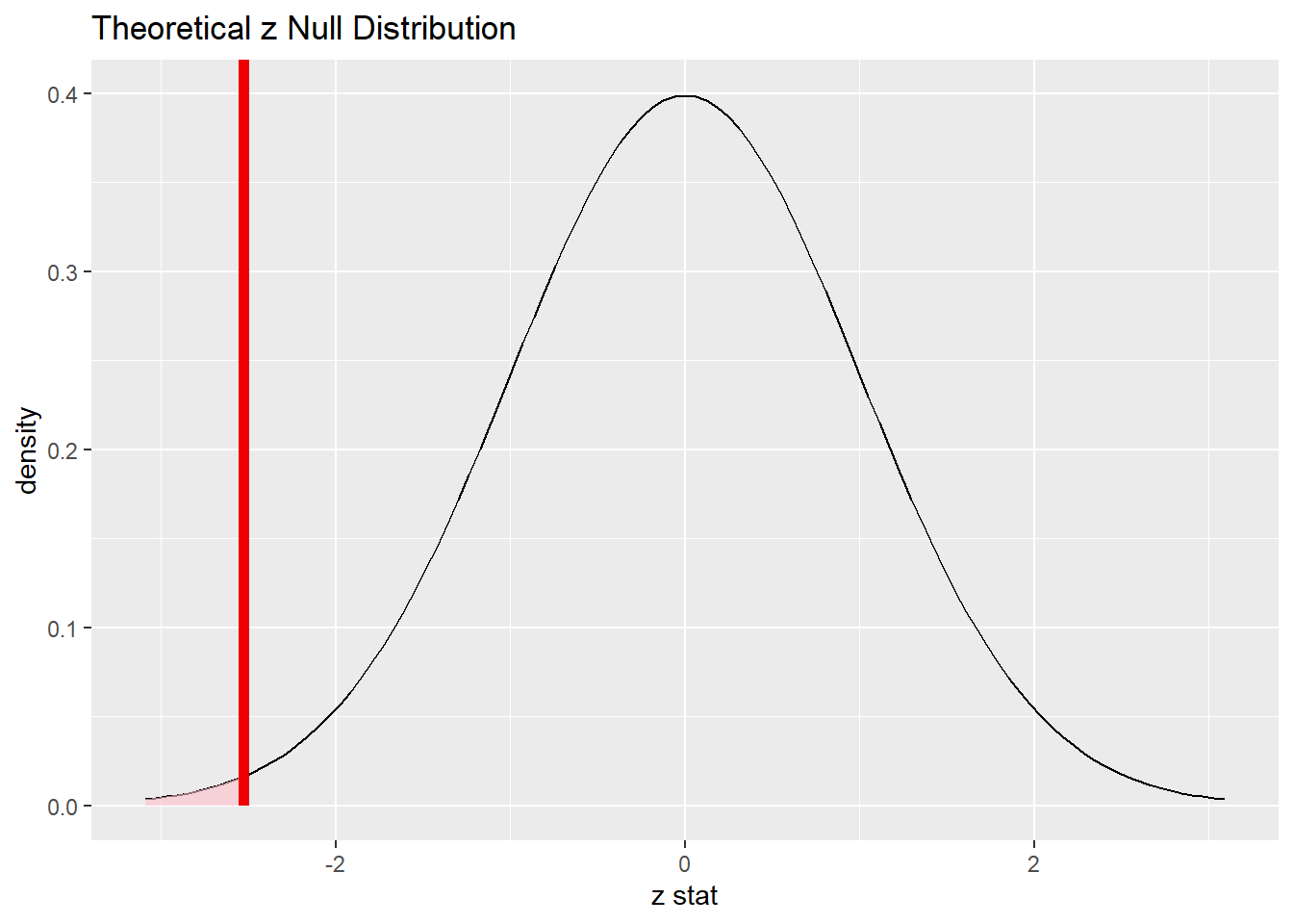
Commentary: In past chapters, we have used the generate verb to get many repetitions (usually 1000) of some kind of random process to simulate the sampling distribution model. In this chapter, we have used the verb assume instead to assume that the sampling distribution is a normal model. As long as the conditions hold, this is a reasonable assumption. This also means that we don’t have to use set.seed as there is no random process to reproduce.
Compare the graph above to what we would see if we simulated the sampling distribution. (Now we do need set.seed!)
set.seed(6789)
alive_test_draw <- heart_transplant2 %>%
    specify(response = survived, success = "alive") %>%
    hypothesize(null = "point", p = 0.5) %>%
    generate(reps = 1000, type = "draw") %>%
    calculate(stat = "prop")
alive_test_draw
alive_test_draw %>%
    visualize() +
    shade_p_value(obs_stat = alive_prop, direction = "less")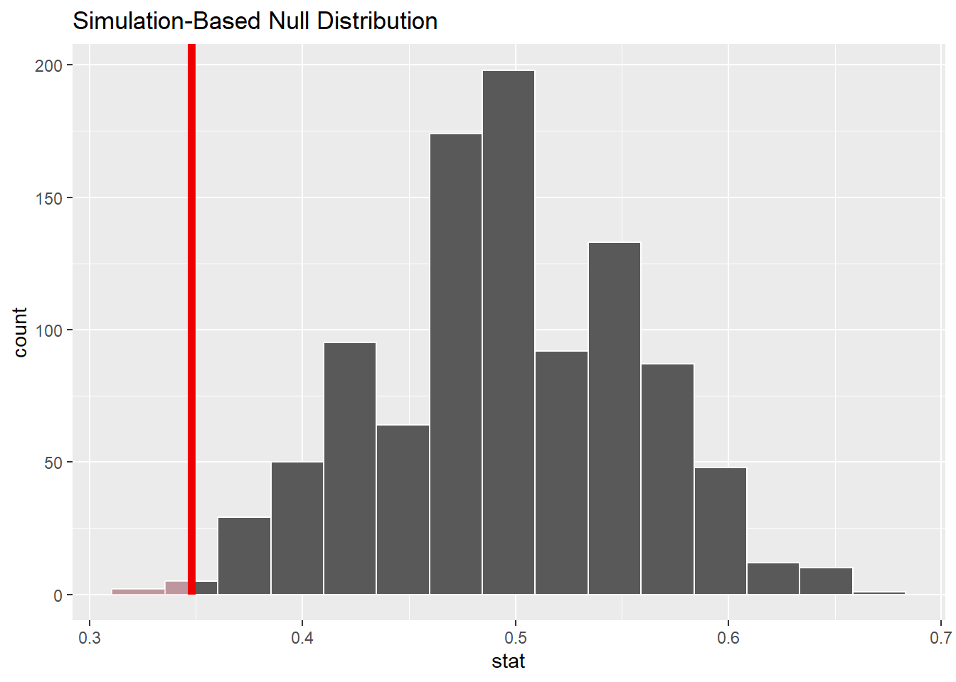
This is essentially the same picture, although the model above is centered on the null value 0.5 instead of the z score of 0. This also means that the obs_stat had to be the sample proportion alive_prop and not the z score alive_z.
15.8.4 Calculate the P-value.
alive_test_p <- alive_test %>%
    get_p_value(obs_stat = alive_z, direction = "less")
alive_test_p
Commentary: compare this to the P-value we get from simulating random draws:
alive_test_draw %>%
    get_p_value(obs_stat = alive_prop, direction = "less")
The values are not exactly the same. And a new simulation with a different seed would likely give another slightly different P-value. The takeaway here is that the P-value itself has some uncertainty, so you should never take the value too seriously.
15.9 Conclusion
15.9.2 State (but do not overstate) a contextually meaningful conclusion.
We have sufficient evidence that heart transplant recipients have less than a 50% chance of survival.
15.9.3 Express reservations or uncertainty about the generalizability of the conclusion.
Because we know nearly nothing about the provenance of the data, it’s hard to generalize the conclusion. We know the data is from 1974, so it’s also very likely that survival rates for heart transplant patients then are not the same as they are today. The most we could hope for is that the Stanford data was representative for heart transplant patients in 1974. Our sample size (69) is also quite small.
15.9.4 Identify the possibility of either a Type I or Type II error and state what making such an error means in the context of the hypotheses.
As we rejected the null, we run the risk of making a Type I error. It is possible that the null is true and that there is a 50% chance of survival for these patients, but we got an unusual sample that appears to have a much smaller chance of survival.
15.10 Confidence interval
15.10.1 Check the relevant conditions to ensure that model assumptions are met.
- Random
- Same as above.
- 10%
- Same as above.
- Success/failure
- There were 24 patients who survived and 45 who died in our sample. Both are larger than 10.
Commentary: In the “Confidence interval” section of the rubric, there is no need to recheck conditions that have already been checked. The sample has not changed; if it met the “Random” and “10%” conditions before, it will meet them now.
So why recheck the success/failure condition?
Keep in mind that in a hypothesis test, we temporarily assume the null is true. The null states that \(p = 0.5\) and the resulting null distribution is, therefore, centered at \(p = 0.5\). The success/failure condition is a condition that applies to the normal model we’re using, and for a hypothesis test, that’s the null model.
By contrast, a confidence interval is making no assumption about the “true” value of \(p\). The inferential goal of a confidence interval is to try to capture the true value of \(p\), so we certainly cannot make any assumptions about it. Therefore, we go back to the original way we learned about the success/failure condition. That is, we check the actual number of successes and failures.
15.10.2 Calculate and graph the confidence interval.
alive_ci <- alive_test %>%
    get_confidence_interval(point_estimate = alive_prop, level = 0.95)
alive_ci
alive_test %>%
    visualize() +
    shade_confidence_interval(endpoints = alive_ci)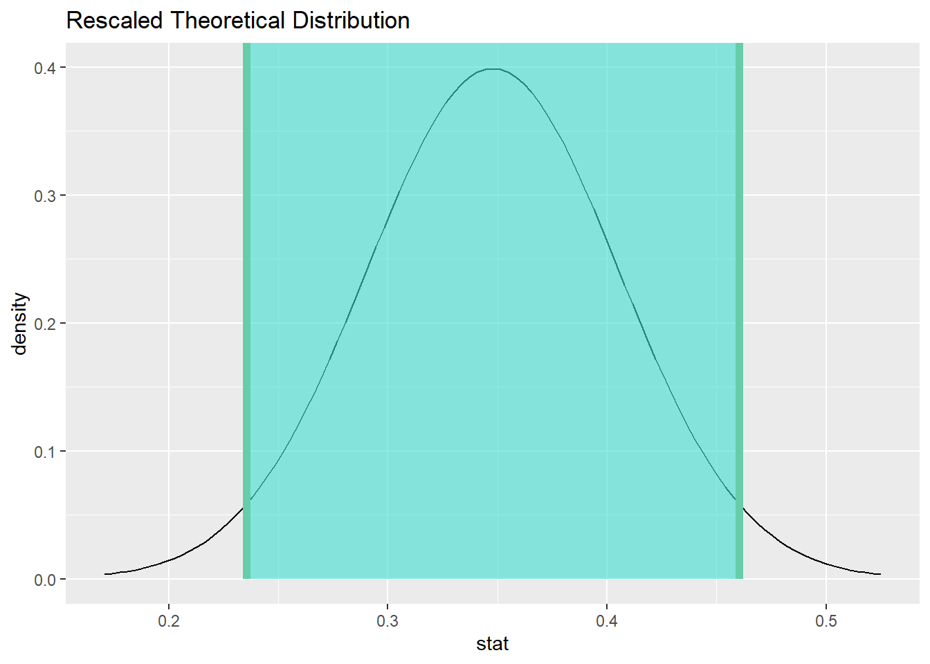
Commentary: when we use a theoretical normal distribution, we have to compute the confidence interval a different way.
When we bootstrapped, we had many repetitions of a process that resulted in a sampling distribution. From all those, we could find the 2.5th percentile and the 97.5th percentile. Although we let the computer do it for us, the process is straightforward enough that we could do it by hand if we needed to. Just put all 1000 bootstrapped values in order, then go to the 25th and 975th position in the list.
We don’t have a list of 1000 values when we use an abstract curve to represent our sampling distribution. Nevertheless, we can find the 2.5th percentile and the 97.5th percentile using the area under the normal curve as we saw in the last two chapters. We can do this “manually” with the qdist command, but we need the standard error first.
Didn’t we calculate this earlier?
\[ SE = \sqrt{\frac{p_{alive}(1 - p_{alive})}{n}} = \sqrt{\frac{0.5(1 - 0.5)}{69}} \]
Well…sort of. The value of \(p_{alive}\) here is the value of the null hypothesis from the hypothesis test above. However, the hypothesis test is done. For a confidence interval, we have no information about any “null” value. There is no null anymore. It’s irrelevant.
So what is the standard error for a confidence interval? Since we don’t have \(p_{alive}\), the best we can do is replace it with \(\hat{p}_{alive}\):
\[ SE = \sqrt{\frac{\hat{p}_{alive} (1 - \hat{p}_{alive})}{n}} = \sqrt{\frac{0.3478261 (1 - 0.3478261 )}{69}}. \]
We can let R do the heavy lifting here:
SE2 <- sqrt(alive_prop * (1 - alive_prop) / 69)
SE2
And now this number can go into qdist as our standard deviation:
## [1] 0.2354468 0.4602054The numbers above are identical to the ones computed by the infer commands.
15.10.3 State (but do not overstate) a contextually meaningful interpretation.
We are 95% confident that the true percentage of heart transplant recipients who survive is captured in the interval (23.5446784%, 46.020539%).
Commentary: Note that when we state our contextually meaningful conclusion, we also convert the decimal proportions to percentages. Humans like percentages a lot better.
15.11 Your turn
Follow the rubric to answer the following research question:
Some heart transplant candidates have already had a prior surgery. Use the variable prior in the heart_transplant data set to determine if fewer than 50% of patients have had a prior surgery. (To be clear, you are being asked to perform a one-sided test again.) Be sure to use the full heart_transplant data, not the modified heart_transplant2 from the previous example.
The rubric outline is reproduced below. You may refer to the worked example above and modify it accordingly. Remember to strip out all the commentary. That is just exposition for your benefit in understanding the steps, but is not meant to form part of the formal inference process.
Another word of warning: the copy/paste process is not a substitute for your brain. You will often need to modify more than just the names of the tibbles and variables to adapt the worked examples to your own work. For example, if you run a two-sided test instead of a one-sided test, there are a few places that have to be adjusted accordingly. Understanding the sampling distribution model and the computation of the P-value goes a long way toward understanding the changes that must be made. Do not blindly copy and paste code without understanding what it does. And you should never copy and paste text. All the sentences and paragraphs you write are expressions of your own analysis. They must reflect your own understanding of the inferential process.
Also, so that your answers here don’t mess up the code chunks above, use new variable names everywhere. In particular, you should use prior_test(instead of alive_test) to store the results of your hypothesis test. Make other corresponding changes as necessary, like prior_test_p instead of alive_test_p, for example.
Exploratory data analysis
Use data documentation (help files, code books, Google, etc.) to determine as much as possible about the data provenance and structure.
Please write up your answer here.
# Add code here to print the data
# Add code here to glimpse the variablesHypotheses
Identify the sample (or samples) and a reasonable population (or populations) of interest.
[Remember that you are using the full heart_transplant data, so your sample size should be larger here than in the example above.]
Please write up your answer here.
Model
Check the relevant conditions to ensure that model assumptions are met.
[Remember that you are using the full heart_transplant data, so the number of successes and failures will be different here than in the example above.]
Please write up your answer here. (Some conditions may require R code as well.)
Conclusion
State (but do not overstate) a contextually meaningful conclusion.
Please write up your answer here.
Confidence interval
Check the relevant conditions to ensure that model assumptions are met.
Please write up your answer here. (Some conditions may require R code as well.)
State (but do not overstate) a contextually meaningful interpretation.
Please write up your answer here.
15.12 Conclusion
When certain conditions are met, we can use a theoretical normal model—a perfectly symmetric bell curve—as a sampling distribution model in hypothesis testing. Because this does not require drawing many samples, it is faster and cleaner than simulation. Of course, on modern computing devices, drawing even thousands of simulated samples is not very time consuming, and the code we write doesn’t really change much. Given the additional success/failure condition that has to met, it’s worth considering the pros and cons of using a normal model instead of simulating the sampling distribution. Similarly, confidence intervals can be obtained directly from the percentiles of the normal model without the need to obtain bootstrapped samples.
15.12.1 Preparing and submitting your assignment
- From the “Run” menu, select “Restart R and Run All Chunks”.
- Deal with any code errors that crop up. Repeat steps 1–-2 until there are no more code errors.
- Spell check your document by clicking the icon with “ABC” and a check mark.
- Hit the “Preview” button one last time to generate the final draft of the
.nb.htmlfile. - Proofread the HTML file carefully. If there are errors, go back and fix them, then repeat steps 1–5 again.
If you have completed this chapter as part of a statistics course, follow the directions you receive from your professor to submit your assignment.