20 Inference for paired data
2.0
20.1 Introduction
In this chapter we will learn how to run inference for two paired numerical variables.
20.1.2 Download the R notebook file
Check the upper-right corner in RStudio to make sure you’re in your intro_stats project. Then click on the following link to download this chapter as an R notebook file (.Rmd).
https://vectorposse.github.io/intro_stats/chapter_downloads/20-inference_for_paired_data.Rmd
Once the file is downloaded, move it to your project folder in RStudio and open it there.
20.2 Load packages
We load the standard tidyverse and infer packages. The openintro package will give access to the textbooks data and the hsb2 data.
## ── Attaching core tidyverse packages ──────────────────────── tidyverse 2.0.0 ──
## ✔ dplyr     1.1.2     ✔ readr     2.1.4
## ✔ forcats   1.0.0     ✔ stringr   1.5.0
## ✔ ggplot2   3.4.2     ✔ tibble    3.2.1
## ✔ lubridate 1.9.2     ✔ tidyr     1.3.0
## ✔ purrr     1.0.2
## ── Conflicts ────────────────────────────────────────── tidyverse_conflicts() ──
## ✖ dplyr::filter() masks stats::filter()
## ✖ dplyr::lag()    masks stats::lag()
## ℹ Use the conflicted package (<http://conflicted.r-lib.org/>) to force all conflicts to become errors## Loading required package: airports
## Loading required package: cherryblossom
## Loading required package: usdata20.3 Paired data
Sometimes data sets have two numerical variables that are related to each other. For example, a diet study might include a pre-weight and a post-weight. The research question is not about either of these variables directly, but rather the difference between the variables, for example how much weight was lost during the diet.
When this is the case, we run inference for paired data. The procedure involves calculating a new variable d that represents the difference of the two paired variables. The null hypothesis is almost always that there is no difference between the paired variables, and that translates into the statement that the average value of d is zero.
20.4 Research question
The textbooks data frame (from the openintro package) has data on the price of books at the UCLA bookstore versus Amazon.com. The question of interest here is whether the campus bookstore charges more than Amazon.
20.5 Inference for paired data
The key idea is that we don’t actually care about the book prices themselves. All we care about is if there is a difference between the prices for each book. These are not two independent variables because each row represents a single book. Therefore, the two measurements are “paired” and should be treated as a single numerical variable of interest, representing the difference between ucla_new and amaz_new.
Since we’re only interested in analyzing the one numerical variable d, this process is nothing more than a one-sample t test. Therefore, there is really nothing new in this chapter.
Let’s go through the rubric.
20.6 Exploratory data analysis
20.6.1 Use data documentation (help files, code books, Google, etc.) to determine as much as possible about the data provenance and structure.
You should type textbooks at the Console to read the help file. The data was collected by a person, David Diez. A quick Google search reveals that he is a statistician who graduated from UCLA. We presume he had access to accurate information about the prices of books at the UCLA bookstore and from Amazon.com at the time the data was collected.
Here is the data set:
textbooks
glimpse(textbooks)## Rows: 73
## Columns: 7
## $ dept_abbr <fct> Am Ind, Anthro, Anthro, Anthro, Art His, Art His, Asia Am, A…
## $ course <fct> C170, 9, 135T, 191HB, M102K, 118E, 187B, 191E, C125, M145B,…
## $ isbn <fct> 978-0803272620, 978-0030119194, 978-0300080643, 978-02262068…
## $ ucla_new <dbl> 27.67, 40.59, 31.68, 16.00, 18.95, 14.95, 24.70, 19.50, 123.…
## $ amaz_new <dbl> 27.95, 31.14, 32.00, 11.52, 14.21, 10.17, 20.06, 16.66, 106.…
## $ more <fct> Y, Y, Y, Y, Y, Y, Y, N, N, Y, Y, N, Y, Y, N, N, N, N, N, N, …
## $ diff <dbl> -0.28, 9.45, -0.32, 4.48, 4.74, 4.78, 4.64, 2.84, 17.59, 3.7…The two paired variables are ucla_new and amaz_new.
20.6.2 Prepare the data for analysis.
Generally, we will need to create a new variable d that represents the difference between the two paired variables of interest. This uses the mutate command that adds an extra column to our data frame. The order of subtraction usually does not matter, but we will want to keep track of that order so that we can interpret our test statistic correctly. In the case of a one-sided test (which this is), it is especially important to keep track of the order of subtraction. Since we suspect the bookstore will charge more than Amazon, let’s subtract in that order. Our hunch is that it will be a positive number, on average.
If you look closely at the tibble above, you will see that there is a column already in our data called diff. It is the same as the column d we just created. So in this case, we didn’t really need to create a new difference variable. However, since most data sets do not come pre-prepared with such a difference variable, it is good to know how to make one if needed.
20.6.3 Make tables or plots to explore the data visually.
Here are summary statistics, a histogram, and a QQ plot for d.
summary(textbooks_d$d)## Min. 1st Qu. Median Mean 3rd Qu. Max.
## -9.53 3.80 8.23 12.76 17.59 66.00
ggplot(textbooks_d, aes(x = d)) +
    geom_histogram(binwidth = 10, boundary = 0)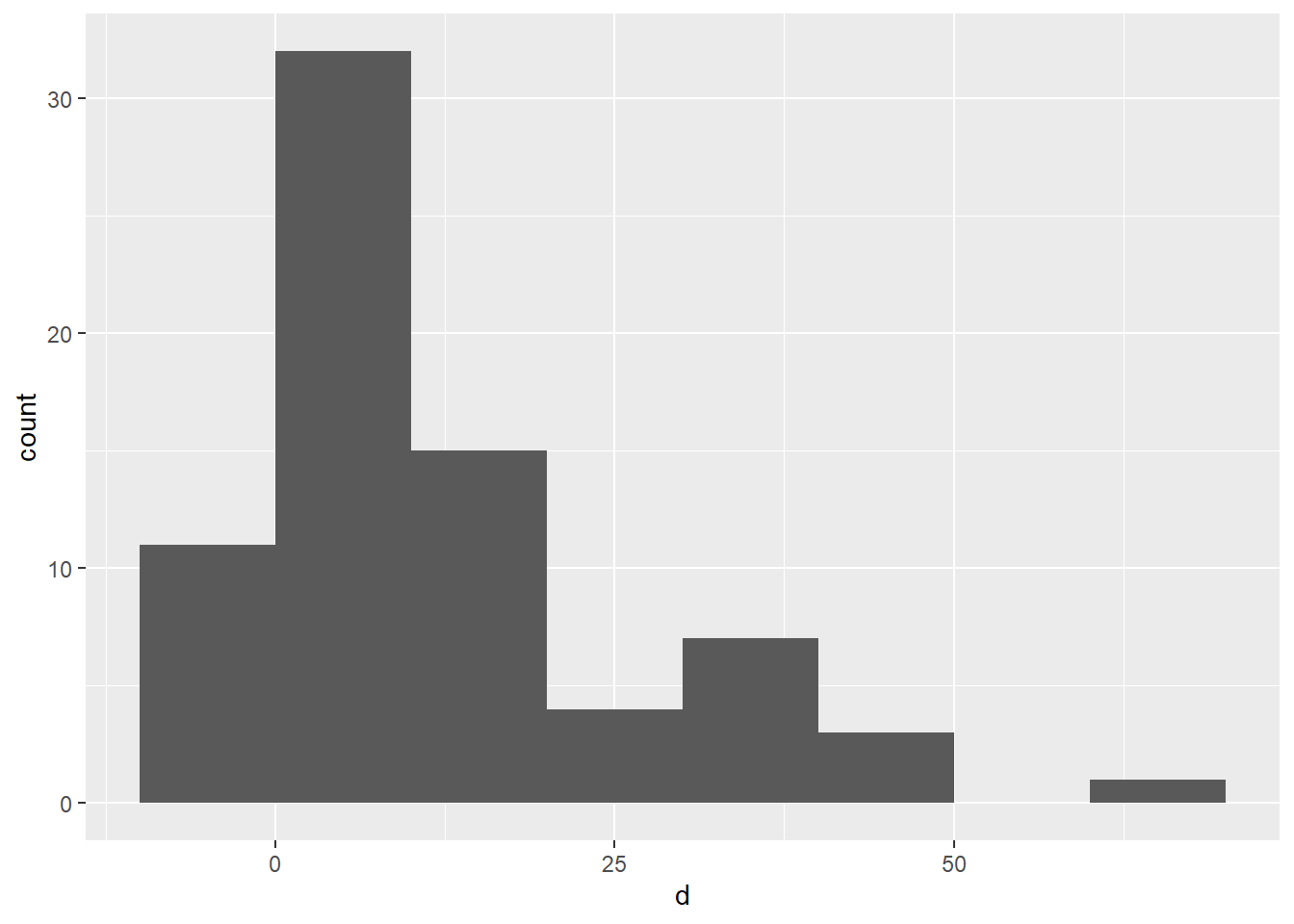
ggplot(textbooks_d, aes(sample = d)) +
    geom_qq() +
    geom_qq_line()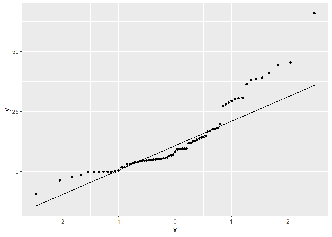
The data is somewhat skewed to the right with one observation that might be a bit of an outlier. If the sample size were much smaller, we might be concerned about this point However, it’s not much higher than other points in that right tail, and it doesn’t appear that its inclusion or exclusion will change the overall conclusion much. If you are concerned that the point might alter the conclusion, run the hypothesis test twice, once with and once without the outlier present to see if the main conclusion changes.
20.7 Hypotheses
20.7.1 Identify the sample (or samples) and a reasonable population (or populations) of interest.
The sample consists of 73 textbooks. The population is all textbooks that might be sold both at the UCLA bookstore and on Amazon.
20.7.2 Express the null and alternative hypotheses as contextually meaningful full sentences.
\(H_{0}:\) There is no difference in textbooks prices between the UCLA bookstore and Amazon.
\(H_{A}:\) Textbook prices at the UCLA bookstore are higher on average than on Amazon.
Commentary: Note we are performing a one-sided test. If we are conducting our own research with our own data, we can decide whether we want to run a two-sided or one-sided test. Remember that we only do the latter when we have a strong hypothesis in advance that the difference should be clearly in one direction and not the other. In this case, it’s not up to us. We have to respect the research question as it was given to us: “The question of interest here is whether the campus bookstore charges more than Amazon.”
20.7.3 Express the null and alternative hypotheses in symbols (when possible).
\(H_{0}: \mu_{d} = 0\)
\(H_{A}: \mu_{d} > 0\)
Commentary: Since we’re really just doing a one-sample t test, we could just call this parameter \(\mu\), but the subscript \(d\) is a good reminder that it’s the mean of the difference variable we care about (as opposed to the mean price of all the books at the UCLA bookstore or the mean price of all the same books on Amazon).
20.8 Model
20.8.2 Check the relevant conditions to ensure that model assumptions are met.
- Random
- We do not know how exactly how David Diez obtained this sample, but the help file claims it is a random sample.
- 10%
- We do not know how many total textbooks were available at the UCLA bookstore at the time the sample was taken, so we do not know if this condition is met. As long as there were at least 730 books, we are okay. We suspect that, based on the size of UCLA and the number of course offerings there, this is a reasonable assumption.
- Nearly normal
- Although the sample distribution is skewed (with a possible mild outlier), the sample size is more than 30.
20.9 Mechanics
20.9.1 Compute the test statistic.
d_t <- textbooks_d %>%
  specify(response = d) %>%
  hypothesize(null = "point", mu = 0) %>%
  calculate(stat = "t")
d_t
20.9.2 Report the test statistic in context (when possible).
The mean difference in textbook prices is 12.7616438.
The value of t is 7.6487711. The mean difference in textbook prices is more than 7 standard errors above a difference of zero.
20.9.3 Plot the null distribution.
## A T distribution with 72 degrees of freedom.
price_test %>%
  visualize() +
  shade_p_value(obs_stat = d_t, direction = "greater")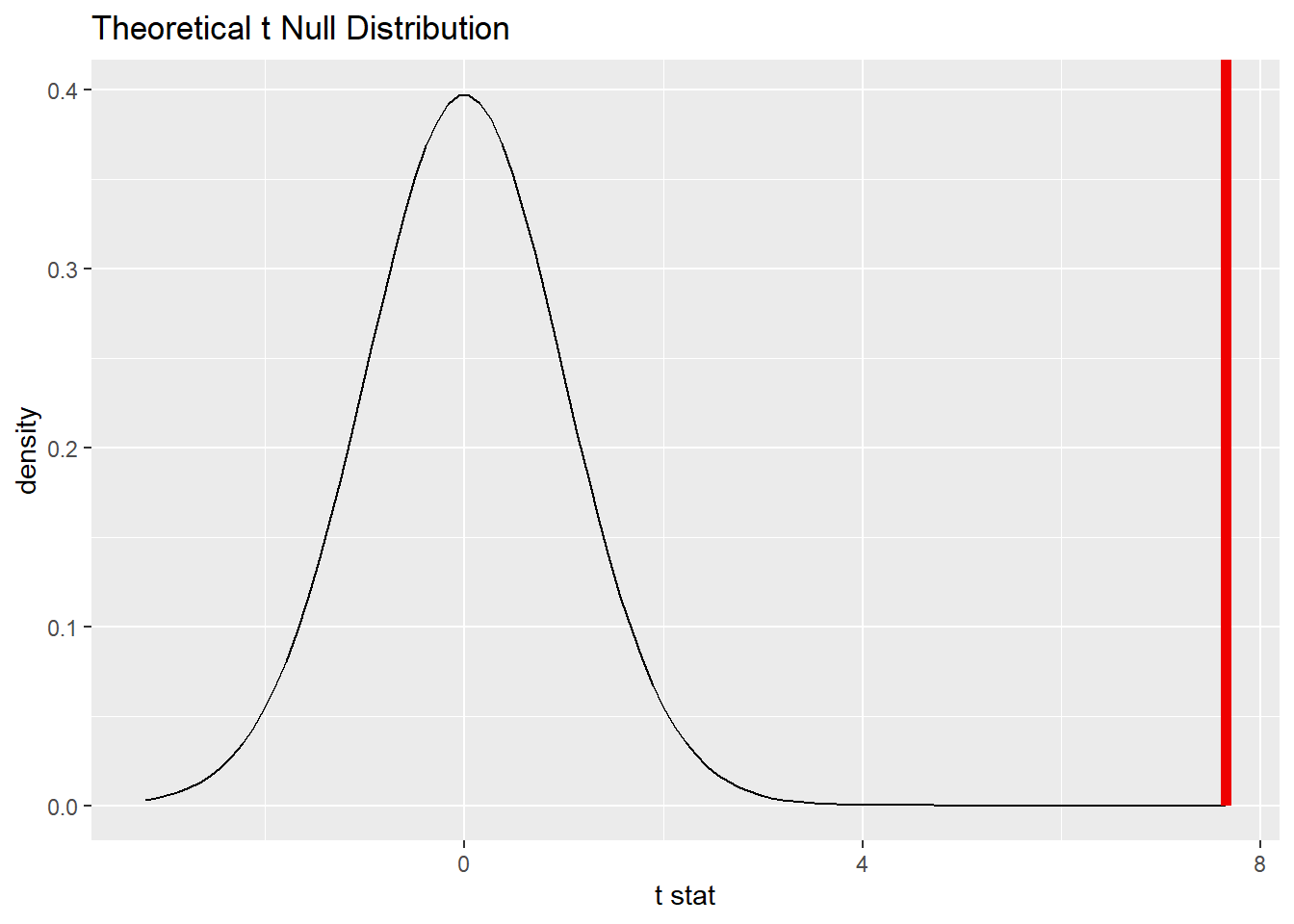
20.9.4 Calculate the P-value.
price_test_p <- price_test %>%
  get_p_value(obs_stat = d_t, direction = "greater")
price_test_p
20.9.5 Interpret the P-value as a probability given the null.
\(P < 0.001\). If there were no difference in textbook prices between the UCLA bookstore and Amazon, there is only a 0% chance of seeing data at least as extreme as what we saw. (Note that the number is so small that it rounds to zero in the inline code above. That zero is technically incorrect. The P-value is never exactly zero. That’s why why also are clear to state \(P < 0.001\).)
20.10 Conclusion
20.10.2 State (but do not overstate) a contextually meaningful conclusion.
We have sufficient evidence that UCLA prices are higher than Amazon prices.
Commentary: Note that because we performed a one-sided test, our conclusion is also one-sided in the hypothesized direction.
20.10.3 Express reservations or uncertainty about the generalizability of the conclusion.
We can be confident about the validity of this data, and therefore the conclusion drawn. We should be careful to limit our conclusion to the UCLA bookstore (and not extrapolate the findings, say, to other campus bookstores.) Depending on when this data was collected, we may not be able to say anything about current prices at the UCLA bookstore either.
20.10.4 Identify the possibility of either a Type I or Type II error and state what making such an error means in the context of the hypotheses.
If we made a Type I error, that would mean there was actually no difference in textbook prices, but that we got an unusual sample that detected a difference.
20.11 Confidence interval
20.11.1 Check the relevant conditions to ensure that model assumptions are met.
All necessary conditions have already been checked.
20.11.2 Calculate and graph the confidence interval.
price_ci <- price_test %>%
  get_confidence_interval(point_estimate = d_mean, level = 0.95)
price_ci
price_test %>%
  visualize() +
  shade_confidence_interval(endpoints = price_ci)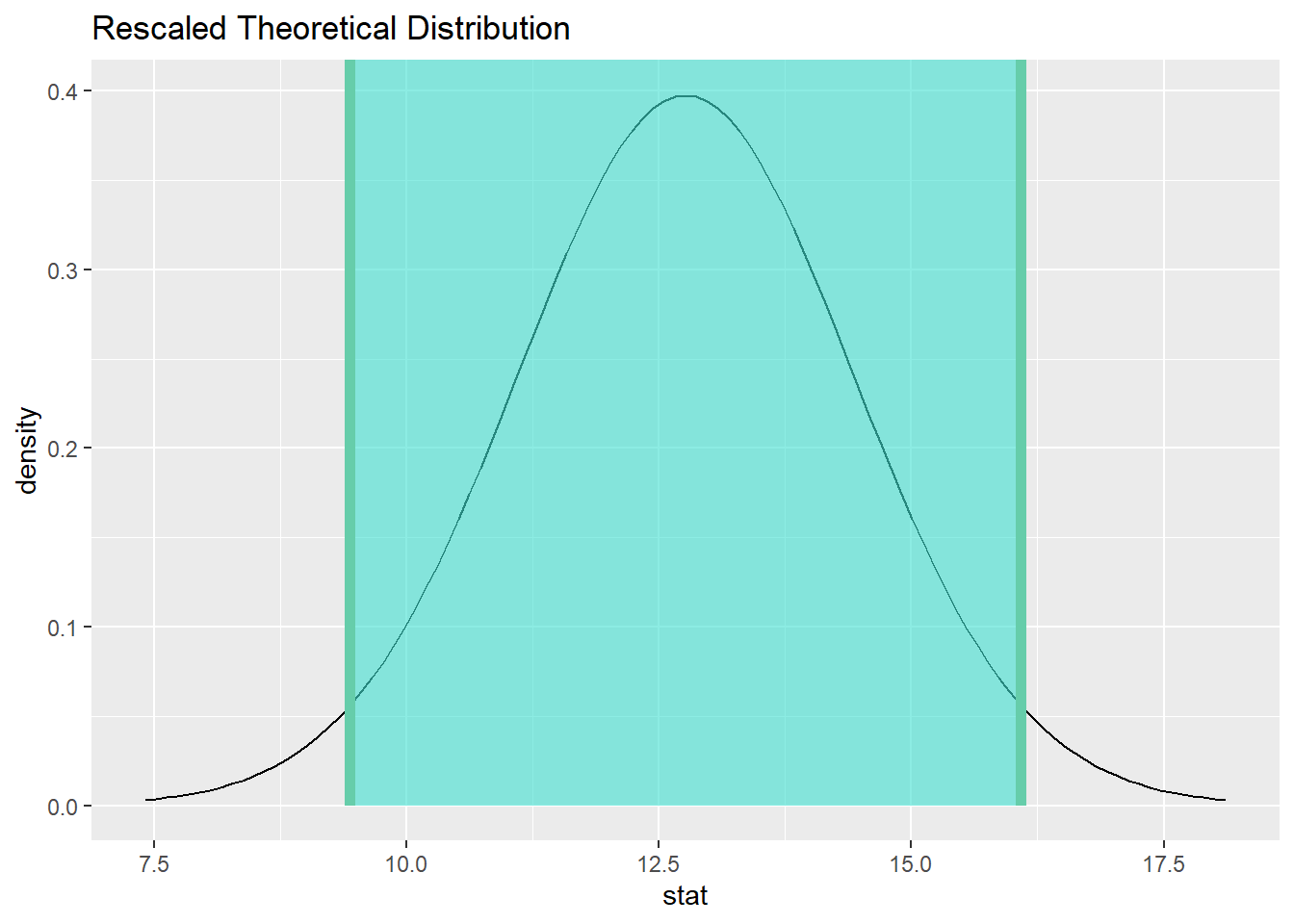
20.11.3 State (but do not overstate) a contextually meaningful interpretation.
We are 95% confident that the true difference in textbook prices between the UCLA bookstore and Amazon is captured in the interval (9.4356361, 16.0876516). This was obtained by subtracting the Amazon price minus the UCLA bookstore. (In other words, since all differences in the confidence interval are positive, all plausible differences indicate that the UCLA prices are higher than the Amazon prices.)
Commentary: Don’t forget that any time we find a number that represents a difference, we have to be clear in the conclusion about the direction of subtraction. Otherwise, we have no idea how to interpret positive and negative values.
20.11.4 If running a two-sided test, explain how the confidence interval reinforces the conclusion of the hypothesis test.
The confidence interval does not contain zero, which means that zero is not a plausible value for the difference textbook prices.
20.11.5 When comparing two groups, comment on the effect size and the practical significance of the result.
To think about the practical significance, imagine that you were a student at UCLA and that every textbook you needed was (on average) $10 to $15 more expensive in the bookstore than purchasing on Amazon. Multiplied across the number of textbooks you need, that could amount to a significant increase in expenses. In other words, that dollar figure is not likely a trivial amount of money for many students who require multiple textbooks each semester.
20.12 Your turn
The hsb2 data set contains data from a random sample of 200 high school seniors from the “High School and Beyond” survey conducted by the National Center of Education Statistics. It contains, among other things, students’ scores on standardized tests in math, reading, writing, science, and social studies. We want to know if students do better on the math test or on the reading test.
Run inference to determine if there is a difference between math scores and reading scores.
The rubric outline is reproduced below. You may refer to the worked example above and modify it accordingly. Remember to strip out all the commentary. That is just exposition for your benefit in understanding the steps, but is not meant to form part of the formal inference process.
Another word of warning: the copy/paste process is not a substitute for your brain. You will often need to modify more than just the names of the data frames and variables to adapt the worked examples to your own work. Do not blindly copy and paste code without understanding what it does. And you should never copy and paste text. All the sentences and paragraphs you write are expressions of your own analysis. They must reflect your own understanding of the inferential process.
Also, so that your answers here don’t mess up the code chunks above, use new variable names everywhere.
Exploratory data analysis
Use data documentation (help files, code books, Google, etc.) to determine as much as possible about the data provenance and structure.
Please write up your answer here
# Add code here to print the data
# Add code here to glimpse the variablesHypotheses
Identify the sample (or samples) and a reasonable population (or populations) of interest.
Please write up your answer here.
Mechanics
Plot the null distribution.
# IF CONDUCTING A SIMULATION...
set.seed(1)
# Add code here to simulate the null distribution.
# Add code here to plot the null distribution.Conclusion
State (but do not overstate) a contextually meaningful conclusion.
Please write up your answer here.
Confidence interval
Check the relevant conditions to ensure that model assumptions are met.
Please write up your answer here. (Some conditions may require R code as well.)
Calculate and graph the confidence interval.
# Add code here to calculate the confidence interval.
# Add code here to graph the confidence interval.State (but do not overstate) a contextually meaningful interpretation.
Please write up your answer here.
20.13 Conclusion
Paired data occurs whenever we have two numerical measurements that are related to each other, whether because they come from the same observational units or from closely related ones. When our data is structured as pairs of measurements in this way, we can subtract the two columns and obtain a difference. That difference variable is the object of our study, and now that it is represented as a single numerical variable, we can apply the one-sample t test from the last chapter.
20.13.1 Preparing and submitting your assignment
- From the “Run” menu, select “Restart R and Run All Chunks”.
- Deal with any code errors that crop up. Repeat steps 1–-2 until there are no more code errors.
- Spell check your document by clicking the icon with “ABC” and a check mark.
- Hit the “Preview” button one last time to generate the final draft of the
.nb.htmlfile. - Proofread the HTML file carefully. If there are errors, go back and fix them, then repeat steps 1–5 again.
If you have completed this chapter as part of a statistics course, follow the directions you receive from your professor to submit your assignment.