3 Covariance
3.1 Calculating covariance
The last chapter was about variance, which measures the spread of a single variable. Now we extend this idea to pairs of variables.
We say that two variables “co-vary” when the spread of one variable is related to the spread of another variable. This relationship represents an association between the two variables.
We’ll call our two variables \(X_{1}\) and \(X_{2}\). To keep things simple, let’s assume that we have already mean centered our variables.
If \(X_{1}\) and \(X_{2}\) are already mean centered, then what are \(\overline{X_{1}}\) and \(\overline{X_{2}}\)?
As we did in the last chapter with variance, we’ll build up the calculation of covariance step-by-step using a table to keep track of intermediate quantities we need.
Here are two variables (with \(n = 7\)) that have been mean centered:
| \(X_{1}\) | \(X_{2}\) | \(\qquad\) | \(\qquad\) |
|---|---|---|---|
| -1 | -2 | ||
| -2 | 2 | ||
| 2 | -2 | ||
| -3 | -1 | ||
| 4 | 2 | ||
| -1 | -2 | ||
| 1 | 3 |
Check that the mean of both columns is truly zero.
Something interesting happens when we look at the product \(X_{1}X_{2}\).
If \(X_{1}\) and \(X_{2}\) both lie above their means, they are both positive numbers. Therefore, their product is positive.
What if both \(X_{1}\) and \(X_{2}\) lie below their means? What do we know about their values individually and what do we know about their product?
Here is the chart again, but with the products listed in a new column:
| \(X_{1}\) | \(X_{2}\) | \(X_{1}X_{2}\) | \(\qquad\) |
|---|---|---|---|
| -1 | -2 | 2 | |
| -2 | 2 | -4 | |
| 2 | -2 | -4 | |
| -3 | -1 | 3 | |
| 4 | 2 | 8 | |
| -1 | -2 | 2 | |
| 1 | 3 | 3 |
Now we add up the products across all seven data pairs:
| \(X_{1}\) | \(X_{2}\) | \(X_{1}X_{2}\) | \(\qquad\) |
|---|---|---|---|
| -1 | -2 | 2 | |
| -2 | 2 | -4 | |
| 2 | -2 | -4 | |
| -3 | -1 | 3 | |
| 4 | 2 | 8 | |
| -1 | -2 | 2 | |
| 1 | 3 | 3 | |
| Sum: 10 |
So when \(X_{1}\) and \(X_{2}\) tend to have similar values (both positive or both negative), their product is usually positive. It’s not true of every pair of values in the table above; some products are negative. But the majority are positive. Therefore, the sum of all such products will be positive.
We’re almost there. Just like we wanted the average squared deviation to calculate the variance, here we want the average of the products from the third column above. And just like in the case of variance, it’s not quite the average we calculate. Instead of dividing by \(n\), we divide by \(n - 1\) for exactly the same esoteric reason. In our example, there are 7 data points (in other words, 7 rows of data), so we divide by 6.
Putting this all together:
| \(X_{1}\) | \(X_{2}\) | \(X_{1}X_{2}\) | \(\quad\) |
|---|---|---|---|
| -1 | -2 | 2 | |
| -2 | 2 | -4 | |
| 2 | -2 | -4 | |
| -3 | -1 | 3 | |
| 4 | 2 | 8 | |
| -1 | -2 | 2 | |
| 1 | 3 | 3 | |
| Sum: 10 | |||
| Covariance: 10/6 = \(\boxed{1.67}\) |
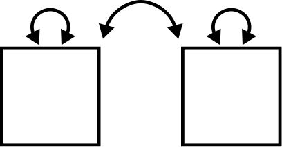
In our diagrams, the covariance of two variables is indicated by a curved, double-headed arrow pointing at both boxes and labeled with the value of the covariance, like this:
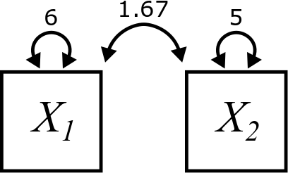
Note that we still include the variances of each of the individual variables. They are still important to us. We just have one new type of arrow now.
Verify that the variances in the diagram are correct for our example. You can do it by hand if you want, but using R is fine too.
Here is the final formula for covariance, written as \(Cov\left(X_{1}, X_{2}\right)\). This works for all pairs of variables, even if they aren’t mean centered. The terms \(\left(X_{1} - \overline{X_1}\right)\) and \(\left(X_{2} - \overline{X_2}\right)\) do the mean centering:
\[ Cov\left(X_{1}, X_{2}\right) = \frac{\sum \left(X_{1} - \overline{X_{1}}\right)\left(X_{2} - \overline{X_{2}}\right)}{n - 1} \]
Suppose \(X_{1}\) tends to be above its mean when \(X_{2}\) is below its mean and \(X_{1}\) tends to be below its mean when \(X_{2}\) is above its mean. What will the product \(\left(X_{1} - \overline{X_{1}}\right)\left(X_{2} - \overline{X_{2}}\right)\) usually be? Therefore, what will the sum of all such products likely be?
For general variables (not necessarily mean centered), the table will actually look like this:
| \(X_{1}\) | \(X_{2}\) | \(\left(X_{1} - \overline{X_{1}}\right)\) | \(\left(X_{2} - \overline{X_{2}}\right)\) | \(\left(X_{1} - \overline{X_{1}}\right)\left(X_{2} - \overline{X_{2}}\right)\) |
|---|---|---|---|---|
| 17 | 23 | -2 | 11 | -22 |
| 25 | 15 | 6 | 3 | 18 |
| … | … | … | … | … |
Calculate the covariance by hand by making a table like the one above. (These variables are not mean centered, so you’ll have to calculate the mean of each variable in order to fill out the third and fourth columns.)
\(X_{3}\): 8, 10, 16, 7, 4, 3
\(X_{4}\): 6, 5, 4, 9, 11, 7
Explain intuitively why the covariance is negative for these two variables.
When calculating variance, the order of the data points does not matter. Why?
When calculating covariance, the order of the data points does matter. Why?
What if you keep pairs together, but rearrange the rows of the table. How does that affect the covariance?
3.2 Calculating covariance in R
Once we’ve done it by hand a few times to make sure we understand how the formula works, from here on out we can let R do the work for us:
## [1] 1.666667## [1] -9.2And here’s some real world data. In addition to temperature (which we’ve already seen), we can use wind speed and see if there is an association between them:
cov(airquality$Temp, airquality$Wind)## [1] -15.272143.3 Covariance rules
We’ll think of the variance and covariance rules as one big list. We left off on Rule 4, so now we’ll introduce Rule 5.
\[ Cov(X, X) = Var(X) \]
In words, Rule 5 states that the covariance of a variable with itself is just the same thing as the variance of that variable. This is quite remarkable! It means that variance is really just a special case of covariance.
Explain why Rule 5 is true. (Hint: think about how you would calculate \(Cov(X, X)\) using either the formula or the table—or both!)
\[ Cov\left(X_{1}, X_{2}\right) = Cov\left(X_{2}, X_{1}\right) \]
In words, we would say that covariance is symmetric.
Explain why Rule 6 is true. (Again, think about the formula or the table—or both!)
The next four rules are analogous to similar rules for variance (Rule 1, Rule 2, Rule 3, and Rule 4).
Suppose that \(C\) is a “constant” variable, meaning that it always has the same value (rather than being a variable that could contain lots of different numbers). Then,
\[ Cov\left(X, C\right) = 0 \]
As always, try to explain this rule. Give an intuitive explanation of why this rule “should” be true. Then think about it computationally, thinking of either the formula or the table—or both!
\[ Cov\left(X_{1} + X_{2}, X_{3}\right) = Cov\left(X_{1}, X_{3}\right) + Cov\left(X_{2}, X_{3}\right) \]
What you should appreciate here is that there is no longer any restriction on the relationships among the variables involved. Rule 2 only worked when the two variables were independent. On the other hand, Rule 8 works for any combination of variables, no matter their relation.
Even more satisfying is this next rule:
\[ Cov\left(X_{1} - X_{2}, X_{3}\right) = Cov\left(X_{1}, X_{3}\right) - Cov\left(X_{2}, X_{3}\right) \]
Yay! The minus sign behaves sensibly now! Of course, since covariances can be positive or negative (unlike variances which are always positive!) we can more safely subtract two of them without worry. And this rule, like Rule 8, does not depend on \(X_{1}\) and \(X_{2}\) being independent. They can be any two variables.
There are versions of these rules with the addition or subtraction on the other side, but these are just minor variations of Rule 8 and Rule 9, so they’re not worth mentioning as a separate rule. Remember that covariance is symmetric, so you can always swap things on the left and right of the comma.
\[ Cov\left(X_{1}, X_{2} \pm X_{3}\right) = Cov\left(X_{1}, X_{2}\right) \pm Cov\left(X_{1}, X_{3}\right) \]
If \(a\) is any number,
\[ Cov\left(a X_{1}, X_{2}\right) = a Cov\left(X_{1}, X_{2}\right) = Cov\left(X_{1}, a X_{2}\right) \]
This rule is also very sensible. Instead of Rule 4 that takes a number \(a\) and pulls out an \(a^{2}\), Rule 10 just pulls out a single factor of \(a\) (from either slot).
Just a couple more rules. We were talking about independence in conjunction with Rule 8 and Rule 9. That leads directly to an interesting and super-important rule:
Why is Rule 11 true, intuitively?
It’s interesting to note that this rule only works one way. In other words, if you know that two variables are independent, then you can conclude their covariance is zero. However, if you know the covariance is zero, that doesn’t necessarily mean that the two variables are independent. We’ll see an example of this later in the chapter.
Finally, one rule to rule them all:
For any two variables \(X_{1}\) and \(X_{2}\):
\[ Var(aX_{1} + bX_{2}) = a^2Var(X_{1}) + b^2Var(X_{2}) + 2abCov(X_{1}, X_{2}) \]
This brings practically everything we know together into one rule!
Proving Rule 12 will give us good practice with the type of manipulation we’ll need to do in future chapters. So here goes. For the first few steps, you name what rule we’re invoking. Then, you’ll pick up the thread and follow it through the last few steps on your own.
\[\begin{align} Var(aX_{1} + bX_{2}) &= Cov(aX_{1} + bX_{2}, aX_{1} + bX_{2}) \\ &= Cov(aX_{1} + bX_{2}, aX_{1}) + Cov(aX_{1} + bX_{2}, bX_{2}) \\ &= Cov(aX_{1}, aX_{1}) + Cov(bX_{2}, aX_{1}) + \\ & \qquad Cov(aX_{1}, bX_{2}) + Cov(bX_{2}, bX_{2}) \\ &= \quad ??? \end{align}\]
You’ll need these rules to do calculations in future chapters. Rather than having to search for them in Chapter 2 and this chapter, we’ve gathered up all the rules in one convenient place in Appendix A.
3.4 Correlation
The pros and cons for calculating covariance are similar to those for variance. The mathematics is much nicer for covariance, but we lose interpretability.
Let’s suppose that \(X_{1}\) measures salary in dollars and \(X_{2}\) measures years of education. We would expect there to be some association between these variables, so we calculate the covariance. What is the unit of measurement of the resulting number?
The solution to the problem here is not as simple as it was for variance. Since variance had squared units, all we had to do was take the square root. Covariance has a weird product of units, so we have to do something more clever.
Following up on the activity above, let’s suppose we have a covariance with units of “dollar-years”. If we divide by a number expressed in dollars, we get rid of those units and we’re left with years. But that seems unsatisfying; covariance should express something about both variables that went into it. Likewise, it makes no sense to divide by a number expressed in years as that would leave us just with dollars.
The solution to the dilemma is to accept that we aren’t going to be able to keep any units in a meaningful way. Therefore, what we want is something standardized, meaning that it has no units.
If \(X_{1}\) is expressed in dollars, can you think of a statistic that measures spread and is also in units of dollars?
Likewise, if \(X_{2}\) is measured in years, what statistic that measures spread is also in units of years?
The previous activity gives us an idea. What if we divide the covariance by both the standard deviation of \(X_{1}\) and the standard deviation of \(X_{2}\)?
\[ \frac{Cov(X_{1},X_{2})}{SD(X_{1}) SD(X_{2})} \]
Sometimes it’s written like this:
\[ \frac{Cov(X_{1},X_{2})}{\sqrt{Var(X_{1})} \sqrt{Var(X_{2})}} \] But that’s the same thing, right?
This quantity has no units. We call this the correlation between \(X_{1}\) and \(X_{2}\). We’ll either write \[ Corr(X_{1}, X_{2}) \] or, if we need to be more concise, \[ r_{X_{1}X_{2}} \]
Yes, this is the same as the correlation coefficient you learned about in your intro stats class, although it wasn’t likely presented to you quite this way.12
One great thing about correlation is that it has no units, so it serves as a sort of “universal” measure of how two variables co-vary. But the best part is that it has a nice intuitive meaning precisely because it factors out the pieces of the covariance that are only there because of the spread of the two variables individually. In other words, the fact that \(X_{1}\) and \(X_{2}\) have their own variability actually complicates the notion of covariance. Those individual variances “corrupt” the interpretation of covariance. But after excising them, all that’s left in the correlation is the “pure” part of the covariance that expresses the relationship or association between \(X_{1}\) and \(X_{2}\).
3.5 Covariance with standardized data
In the last chapter, you showed that the variance of a standardized variable was 1. What is the covariance between two standardized variables?
Let’s standardize both \(X_{1}\) and \(X_{2}\). To make the math a little easier, we’ll use similar notation to what we used at the end of the last chapter.
\(M_{1} = \overline{X_{1}}\)
\(S_{1} = SD(X_{1})\)
\(M_{2} = \overline{X_{2}}\)
\(S_{2} = SD(X_{2})\)
And we’ll write the z-scores in a way that is more amenable to mathematical manipulation (like before):
\[ Z_{1} = \frac{1}{S_{1}}\left(X_{1} - M_{1}\right) \]
\[ Z_{2} = \frac{1}{S_{2}}\left(X_{2} - M_{2}\right) \]
This looks a little more intimidating, but if you apply the rules, it works out:
\[\begin{align} Cov(Z_{1}, Z_{2}) &= Cov\left( \frac{1}{S_{1}}\left(X_{1} - M_{1}\right), \frac{1}{S_{2}}\left(X_{2} - M_{2}\right) \right) \\ &= \quad ??? \end{align}\]
Work this out. Take your time. Apply the rules carefully. So that you know what you’re aiming for, you should get
\[ Cov(Z_{1}, Z_{2}) = \frac{Cov\left( X_{1}, X_{2} \right)}{S_{1} S_{2}} \]
Okay, now remember that \(S_{1}\) is just a convenient substitute for \(SD(X_{1})\) and \(S_{2}\) is just a substitute for \(SD(X_{2})\). Wait, does that answer look familiar?
This is cool! Correlation is simply the covariance of two variables after they’ve been standardized.
This also reinforces the earlier comment about interpreting covariance after removing the extraneous influence of the spread of the individual variables. Standardizing variables makes the spread of all variables 1, so their covariance is now a pure representation of just the association between them.
You probably remember from intro stats that correlation takes on values between -1 and 1. That fact is not obvious from the formula we have. Why should the fraction \[ \frac{Cov(X_{1},X_{2})}{SD(X_{1}) SD(X_{2})} \] be bounded by -1 and 1?
Let’s go back to standardized variable to keep things simple. The correlation is just the covariance of two standardized variables:
\[ Corr(X_{1}, X_{2}) = Cov(Z_{1}, Z_{2}) \]
Use the rules to calculate this:
\[ Var(Z_{1} + Z_{2}) \]
Remember that \(Z_{1}\) and \(Z_{2}\) are not necessarily independent. (In fact, we hope they are not. Otherwise, why do we care about their correlation? It would be zero!) So you need Rule 12, not Rule 2. Keep manipulating until you get \[ 2 + 2Corr(X_{1}, X_{2}) \]
Since variances are always non-negative, we now know that
\[ 0 \leq 2 + 2Corr(X_{1}, X_{2}) \] Solve this inequality for \(Corr(X_{1}, X_{2})\).
Now follow the exact same steps for \[ Var(Z_{1} - Z_{2}) \]
Very little should change in your answer, but there is one small change. Again, solve the resulting inequality. (Don’t forget the key rule when working with inequalities that multiplying or dividing by a negative number changes the direction of the inequality.)
Here is a fact we will state without proof:
Correlations are only interpretable as the strength of linear associations.
Why is this? Basically, it boils down to the fact that a “perfect” correlation of 1 or -1 is only achievable when data points lie on a perfectly straight line. Therefore, thinking of correlation as lying between 0 and 1 (or 0 and -1) is only sensible if you are judging how close points are to lying on a straight line. We’ll see examples of this in the next section when we plot some data.
To calculation correlation in R, use the cor command:
cor(airquality$Temp, airquality$Wind)## [1] -0.4579879Use R to confirm that the number above is the covariance divided by the product of the standard deviations.
3.6 Visualizing correlation
Covariance is hard to interpret, so when we’re visualizing data and we want to understand any association that might exist between two variables, correlation is a much better statistic to calculate. Let’s see how correlation relates to the graph of two variables.
Before getting into the graphing, we will need to load some packages. The tidyverse is a whole set of commonly used packages that will allow us to work with data frames (or “tibbles” as the cool kids are calling them) and make graphs. Be sure to load the package by typing the following in R before going any further:
## ── Attaching packages ─────────────────────────────────────── tidyverse 1.3.1 ──## ✔ ggplot2 3.3.6 ✔ purrr 0.3.4
## ✔ tibble 3.1.7 ✔ dplyr 1.0.9
## ✔ tidyr 1.2.0 ✔ stringr 1.4.0
## ✔ readr 2.1.2 ✔ forcats 0.5.1## ── Conflicts ────────────────────────────────────────── tidyverse_conflicts() ──
## ✖ dplyr::filter() masks stats::filter()
## ✖ dplyr::lag() masks stats::lag()In fact, from here on out, we’ll start each chapter by loading any necessary libraries in R that we’ll need.
The standard graph of two numerical variables is a scatterplot. Let’s start with a straight line relationship. First, we define two variables. We’ll use some shortcuts here to make our lives a little easier. The seq command just generates a sequence of numbers.
X5 <- seq(1, 9)
X5
## [1] 1 2 3 4 5 6 7 8 9Then we can establish a linear relationship just by declaring one in a formula:
X6 <- 3 + 0.5 * X5
X6
## [1] 3.5 4.0 4.5 5.0 5.5 6.0 6.5 7.0 7.5To put both variables into the same graph, it helps to make them both columns in a single tibble.
linear_data <- tibble(X5, X6)
linear_data
## # A tibble: 9 × 2
## X5 X6
## <int> <dbl>
## 1 1 3.5
## 2 2 4
## 3 3 4.5
## 4 4 5
## 5 5 5.5
## 6 6 6
## 7 7 6.5
## 8 8 7
## 9 9 7.5And here is the graph:
ggplot(linear_data, aes(y = X6, x = X5)) +
    geom_point()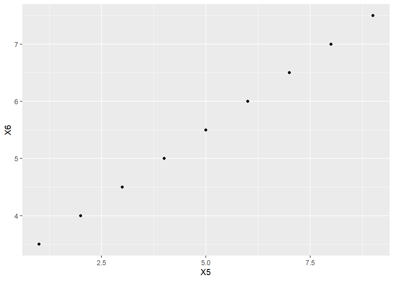
Now the correlation:
cor(X5, X6)## [1] 1It is 1, as expected.
What about a perfectly straight line with a negative slope?
X7 <- 5 - 0.2 * X5
X7
## [1] 4.8 4.6 4.4 4.2 4.0 3.8 3.6 3.4 3.2We’ll throw this new variable into the tibble we already have (for convenience). To explain the syntax below, the %>% symbol is called a “pipe” and it tells R to pass the linear_data tibble on to the next row to process it. And the processing itself is dictated by the bind_cols command which tells R to “bind a new column” to the tibble. The part that says X7 = X7 may be a little confusing. It says to add the new column X7, but also still call it X7.
## # A tibble: 9 × 3
##      X5    X6    X7
##   <int> <dbl> <dbl>
## 1     1   3.5   4.8
## 2     2   4     4.6
## 3     3   4.5   4.4
## 4     4   5     4.2
## 5     5   5.5   4
## 6     6   6     3.8
## 7     7   6.5   3.6
## 8     8   7     3.4
## 9     9   7.5   3.2
ggplot(linear_data, aes(y = X7, x = X5)) +
    geom_point()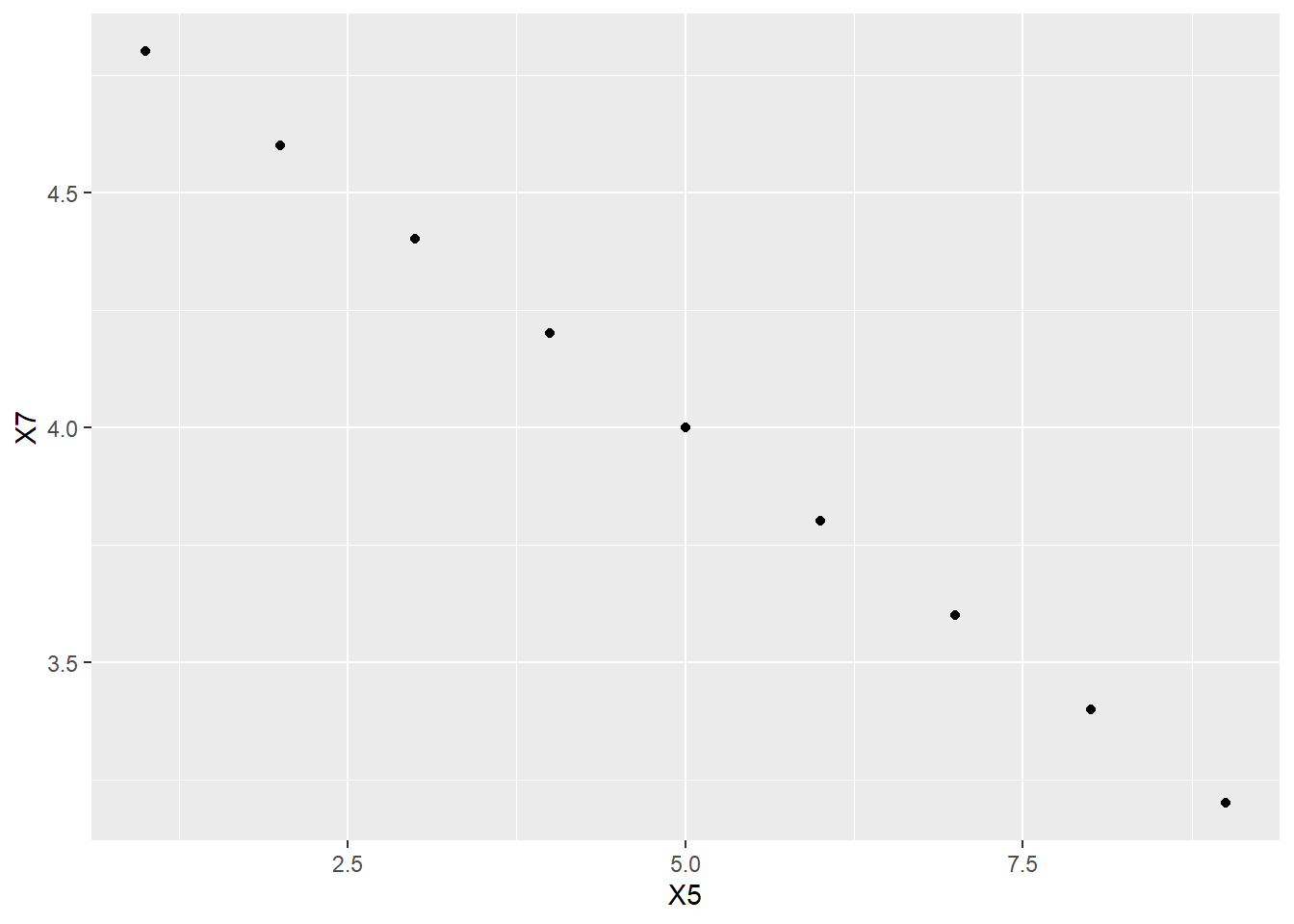
cor(X5, X7)## [1] -1Again, that is what we expected.
What happens if we plot random data? The runif command just chooses random numbers uniformly between 0 and 1.13 We use set.seed to make our work reproducible. You will get the same set of random numbers on your machine if you use the same seed as we use here.
X8## [1] 0.113703411 0.622299405 0.609274733 0.623379442 0.860915384 0.640310605
## [7] 0.009495756 0.232550506 0.666083758 0.514251141 0.693591292 0.544974836
## [13] 0.282733584 0.923433484 0.292315840 0.837295628 0.286223285 0.266820780
## [19] 0.186722790 0.232225911
X9## [1] 0.31661245 0.30269337 0.15904600 0.03999592 0.21879954 0.81059855
## [7] 0.52569755 0.91465817 0.83134505 0.04577026 0.45609148 0.26518667
## [13] 0.30467220 0.50730687 0.18109621 0.75967064 0.20124804 0.25880982
## [19] 0.99215042 0.80735234
random_data <- tibble(X8, X9)
random_data
## # A tibble: 20 × 2
## X8 X9
## <dbl> <dbl>
## 1 0.114 0.317
## 2 0.622 0.303
## 3 0.609 0.159
## 4 0.623 0.0400
## 5 0.861 0.219
## 6 0.640 0.811
## 7 0.00950 0.526
## 8 0.233 0.915
## 9 0.666 0.831
## 10 0.514 0.0458
## 11 0.694 0.456
## 12 0.545 0.265
## 13 0.283 0.305
## 14 0.923 0.507
## 15 0.292 0.181
## 16 0.837 0.760
## 17 0.286 0.201
## 18 0.267 0.259
## 19 0.187 0.992
## 20 0.232 0.807
ggplot(random_data, aes(y = X9, x = X8)) +
    geom_point()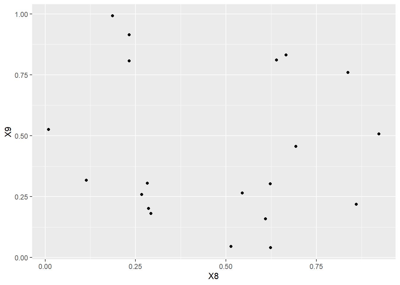
What do you guess is the correlation between \(X_{8}\) and \(X_{9}\)?
Now calculate it using R? Did you get the exact answer you guessed? If not, why not?
What about data that follows a perfect mathematical relationship that is not a straight line? For example, here is a part of a parabola.
X10 <- 0.1 * X5^2
X10
## [1] 0.1 0.4 0.9 1.6 2.5 3.6 4.9 6.4 8.1
nonlinear_data <- tibble(X5, X10)
nonlinear_data
## # A tibble: 9 × 2
## X5 X10
## <int> <dbl>
## 1 1 0.1
## 2 2 0.4
## 3 3 0.9
## 4 4 1.6
## 5 5 2.5
## 6 6 3.6
## 7 7 4.9
## 8 8 6.4
## 9 9 8.1
ggplot(nonlinear_data, aes(y = X10, x = X5)) +
    geom_point()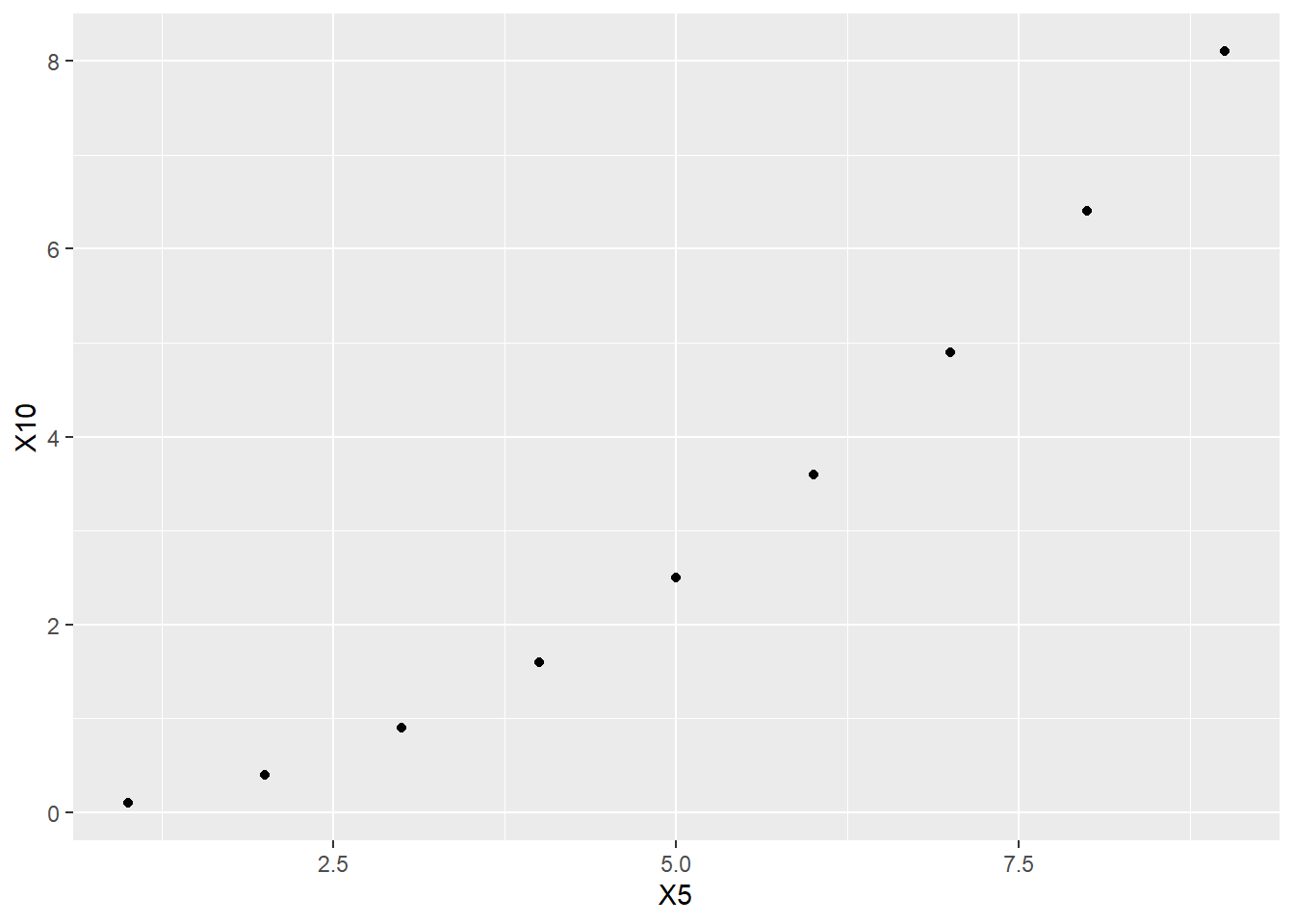
Now for the correlation:
cor(X5, X10)## [1] 0.975281This is a large correlation, but it is not exactly 1, even though the points follow a precise mathematical relationship. That relationship is not linear.
Here’s a fascinating example. For this, we’ll want a parabola that goes down and then up.
X11 <- 0.5 * (X5 - 5)^2
X11
## [1] 8.0 4.5 2.0 0.5 0.0 0.5 2.0 4.5 8.0## # A tibble: 9 × 3
## X5 X10 X11
## <int> <dbl> <dbl>
## 1 1 0.1 8
## 2 2 0.4 4.5
## 3 3 0.9 2
## 4 4 1.6 0.5
## 5 5 2.5 0
## 6 6 3.6 0.5
## 7 7 4.9 2
## 8 8 6.4 4.5
## 9 9 8.1 8
ggplot(nonlinear_data, aes(y = X11, x = X5)) +
    geom_point()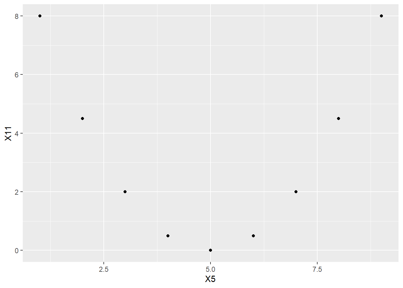
Before looking at the answer, what is your guess for the correlation between \(X_{5}\) and \(X_{11}\)?
Now calculate the correlation in R.
Again, there’s a perfect mathematical relationship between these two variables. They are most definitely associated. So why is the correlation 0?
Recall the earlier promise to discuss Rule 11. If two variables are independent, then their covariance is zero, and, therefore, their correlation is also zero. However, this rule doesn’t work the other way around. The claim is that knowing the covariance/correlation is zero does not imply (necessarily) that the two variables are independent. Here is the promised example of that phenomenon. \(X_{5}\) and \(X_{11}\) have zero correlation. And yet, \(X_{5}\) and \(X_{11}\) are definitely not independent.
This is important enough for a fancy box:
When you see that the correlation between two variables is zero or near zero, be careful not to conclude that the variables are independent.
A zero or near-zero correlation indicates only the lack of a linear association between two variables. There may be nonlinear associations. That’s why it’s always a good idea to graph your data.
Real data is, of course, much messier and it’s just not possible to have perfect correlations between two variables measured out there in the real world. (If you do find a perfect correlation between two columns of your data, chances are that you either recorded the same column twice, or the second column is some simple transformation of first column, like multiplying every value by the same number or something like that.)
Here is a plot of the temperature (degrees Fahrenheit) and wind speed (mph) from the New York air quality data set.
ggplot(airquality, aes(y = Temp, x = Wind)) +
    geom_point()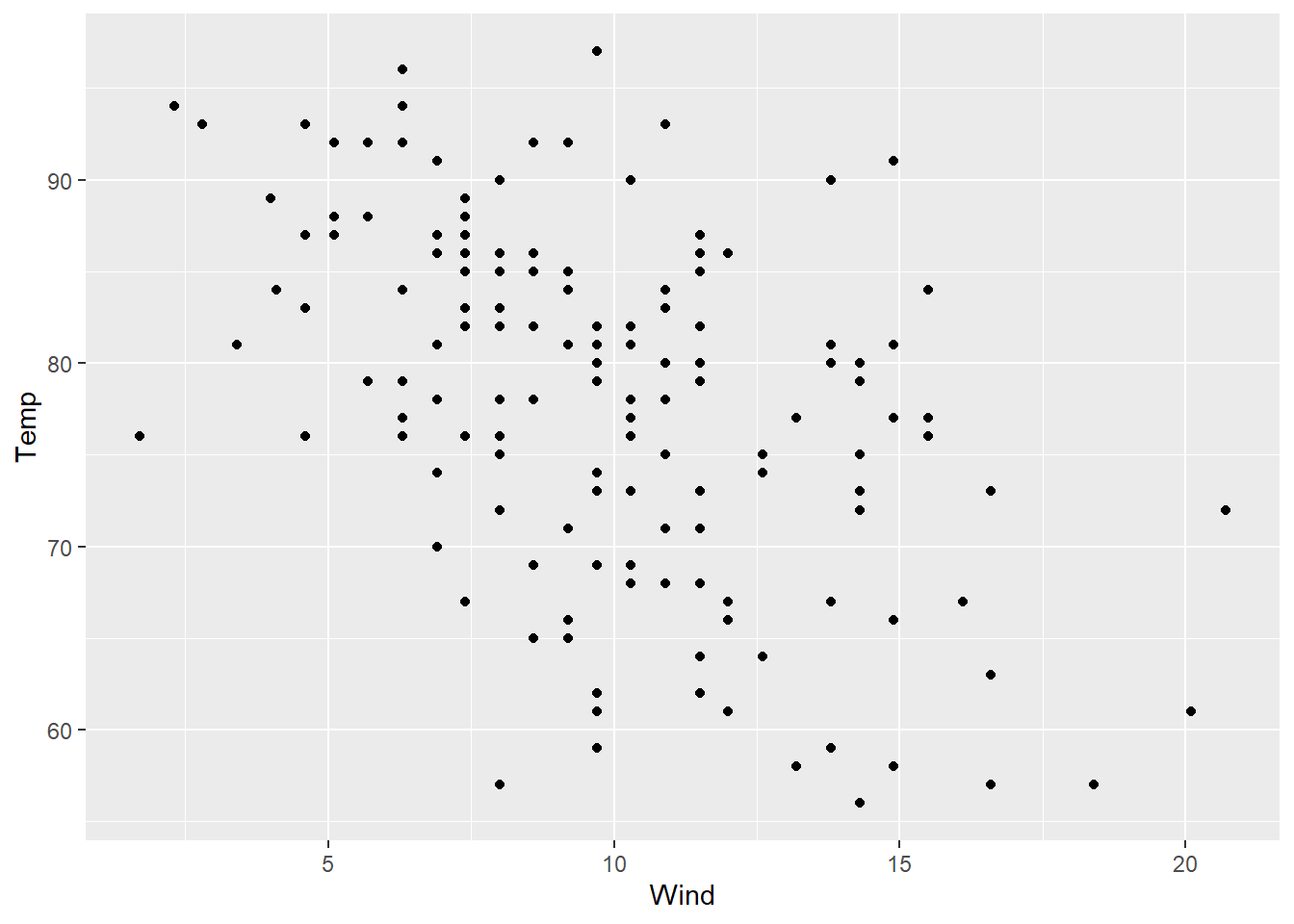
Just looking at the scatterplot (without calculating anything), is the correlation between these two variables positive or negative? Try guessing the exact value of the correlation.
Now calculate the exact value of the correlation to see how close you were.
If you want some practice with looking at scatterplots and guessing the correlation, try this online game:
Turn up the sound! If the whole class plays at the same time, your classroom will sound like an arcade. Compete with your classmates to see who can get the high score.